by Shehrzad Qureshi
Senior Engineer, BDTI
May 14, 2011

A typical processing pipeline for computer vision is given in Figure 1 below:

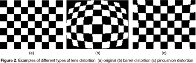
The focus of this article is on the lens correction block. In less than ideal optical systems, like those which will be found in cheaper smartphones and tablets, incoming frames will tend to get distorted along their edges. The most common types of lens distortions are either barrel distortion, pincushion distortion, or some combination of the two^[1]. Figure 2 is an illustration of the types of distortion encountered in vision, and in this article we will discuss strategies and implementations for correcting for this type of lens distortion.

These types of lens aberrations can cause problems for vision algorithms because machine vision usually prefers straight edges (for example lane finding in automotive, or various inspection systems). The general effect of both barrel and pincushion distortion is to project what should be straight lines as curves. Correcting for these distortions is computationally expensive because it is a per-pixel operation. However the correction process is also highly regular and “embarassingly data parallel” which makes it amenable to FPGA or GPU acceleration. The FPGA solution can be particularly attractive as there are now cameras on the market with FPGAs in the camera itself that can be programmed to perform this type of processing^[2].

Calibration Procedure

The rectlinear correction procedure can be summarized as warping a distorted image (see Figure 2b and 2c) to remove the lens distortion, thus taking the frame back to its undistorted projection (Figure 2a). In other words, we must first estimate the lens distortion function, and then invert it so as to compensate the incoming image frame. The compensated image will be referred to as theundistorted image.

Both types of lens aberrations discussed so far are radial distortions that increase in magnitude as we move farther away from the image center. In order to correct for this distortion at runtime, we first must estimate the coefficients of a parameterized form of the distortion function during a calibration procedure that is specific to a given optics train. The detailed mathematics behind this parameterization is beyond the scope of this article, and is covered thoroughly elsewhere^[3]. Suffice it to say if we have:

where:

• = original distorted point coordinates
• = image center
• = undistorted (corrected) point coordinates

then the goal is to measure the distortion model where:

and:

The purpose of the calibration procedure is to estimate the radial distortion coefficients which can be achieved using a gradient descent optimizer^[3]. Typically one images a test pattern with co-linear features that are easily extracted autonomously with sub-pixel accuracy. The checkerboard in Figure 2a is one such test pattern that the author has used several times in the past. Figure 3 summarizes the calibration process:

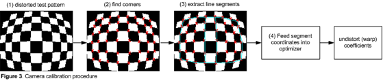
The basic idea is to image a distorted test pattern, extract the coordinates of lines which are known to be straight, feed these coordinates into an optimizer such as the one described in^[3], which emits the lens undistort warp coefficients. These coefficients are used at run-time to correct for the measured lens distortion.

In the provided example we can use a Harris corner detector to automatically find the corners of the checkerboard pattern. The OpenCV library has a robust corner detection function that can be used for this purpose^[4]. The following snippet of OpenCV code can be used to extract the interior corners of the calibration image of Figure 2a:

const int nSquaresAcross=9;
const int nSquaresDown=7;
const int nCorners=(nSquaresAcross-1)*(nSquaresDown-1);
CvSize szcorners = cvSize(nSquaresAcross-1,nSquaresDown-1);
std::vector<CvPoint2D32f> vCornerList(nCorners);
/* find corners to pixel accuracy */
int cornerCount = 0;
const int N = cvFindChessboardCorners(pImg, /* IplImage */
szcorners,
&vCornerList[0],
&cornerCount);
/* should check that cornerCount==nCorners */
/* sub-pixel refinement */
cvFindCornerSubPix(pImg,
&vCornerList[0],
cornerCount,
vSize(5,5),
cvSize(-1,-1),
cvTermCriteria(CV_TERMCRIT_EPS,0,.001));

Segments corresponding to what should be straight lines are then constructed from the point coordinates stored in the STL vCornerList container. For the best results, multiple lines should be used and it is necessary to have both vertical and horizontal line segments for the optimization procedure to converge to a viable solution (see the blue lines in Figure 3).

Finally, we are ready to determine the radial distortion coefficients. There are numerous camera calibration packages (including one in OpenCV), but a particularly good open-source ANSI C library can be locatedhere^[5]. Essentially the line segment coordinates are fed into an optimizer which determines the undistort coefficients by minimizing the error between the radial distortion model and the training data. These coefficients can then be stored in a lookup table for run-time image correction.

Lens Distortion Correction (Warping)

The referenced calibration library^[5] also includes a very informativeonline demo. The demo illustrates the procedure briefly described here. Application of the radial distortion coefficients to correct for the lens aberrations basically boils down an image warp operation. That is, for each pixel in the (undistorted) frame, we compute the distance from the image center and evaluate a polynomial that gives us the pixel coordinates from which to fill in the corrected pixel intensity. Because the polynomial evaluation will more than likely fall in between integer pixel coordinates, some form of interpolation must be used. The simplest and cheapest interpolant is so-called “nearest neighbor” which as its name implies means to simply pick the nearest pixel, but this technique results in poor image quality. At a bare minimum bilinear interpolation should be employed and oftentimes higher order bicubic interpolants are called for.

The amount of computations per frame can become quite large, particularly if we are dealing with color frames. The saving grace of this operation is its inherent parallelism (each pixel is completely independent of its neighbors and hence can be corrected in parallel). This parallelism and the highly regular nature of the computations lends itself readily to accelerators, either via FPGAs^[6,7] or GPUs^[8,9]. The source code provided in^[5] includes a lens correction function with full ANSI C source.

A faster software implementation than ^[5] can be realized using the OpenCVcvRemap() function^[4]. The input arguments into this function are the source and destination images, the source to destination pixel mapping (expressed as two floating point arrays), interpolation options, and a default fill value (if there are any holes in the rectilinear corrected image). At calibration time, we evaluate the distortion model polynomials just once and then store the pixel mapping to disk or memory. At run-time the software simply callscvRemap()—which is optimized and can accommodate color frames—to correct the lens distortion.

References

[1] Wikipedia page:  http://en.wikipedia.org/wiki/Distortion_(optics)

[2] http://www.hunteng.co.uk/info/fpgaimaging.htm

[3] L. Alvarez, L. Gomez, R. Sendra. An Algebraic Approach to Lens Distortion by Line Rectification, Journal of Mathematical Imaging and Vision, Vol. 39 (1), July 2009, pp. 36-50.

[4] Bradski, Gary and Kaebler, Adrian. Learning OpenCV (Computer Vision with the OpenCV Library), O’Reilly, 2008.

[5] http://www.ipol.im/pub/algo/ags_algebraic_lens_distortion_estimation/

[6] Daloukas, K.; Antonopoulos, C.D.; Bellas, N.; Chai, S.M. “Fisheye lens distortion correction on multicore and hardware accelerator platforms,”Parallel & Distributed Processing (IPDPS), 2010 IEEE International Symposium on , vol., no., pp.1-10, 19-23 April 2010

[7] J. Jiang , S. Schmidt , W. Luk and D. Rueckert “Parameterizing reconfigurable designs for image warping”,Proc. SPIE, vol. 4867, pp. 86 2002.

[8] http://visionexperts.blogspot.com/2010/07/image-warping-using-texture-fetches.html

[9] Rosner,J., Fassold,H., Bailer,W., Schallauer,P.: “Fast GPU-based Image Warping and Inpainting for Frame Interpolation”, Proceedings of Computer Graphics, Computer Vision and Mathematics (GraVisMa) Workshop, Plzen, CZ, 2010