
大家好,又见面了,我是你们的朋友全栈君。如果您正在找激活码,请点击查看最新教程,关注关注公众号 “全栈程序员社区” 获取激活教程,可能之前旧版本教程已经失效.最新Idea2022.1教程亲测有效,一键激活。
Jetbrains全系列IDE稳定放心使用
SIFT简介
整理一下方便阅读,作者写的东西摘自论文,在此感谢xiaowei等的贡献
- DoG尺度空间构造(Scale-space extrema detection)http://blog.csdn.net/xiaowei_cqu/article/details/8067881
- 关键点搜索与定位(Keypoint localization)http://blog.csdn.net/xiaowei_cqu/article/details/8087239
- 方向赋值(Orientation assignment)http://blog.csdn.net/xiaowei_cqu/article/details/8096072
- 关键点描述(Keypoint descriptor)http://blog.csdn.net/xiaowei_cqu/article/details/8113565
- OpenCV实现:特征检测器FeatureDetectorhttp://blog.csdn.net/xiaowei_cqu/article/details/8652096
- SIFT中LoG和DoG的比较http://blog.csdn.net/xiaowei_cqu/article/details/27692123
DoG尺度空间构造
尺度空间中各尺度图像的模糊程度逐渐变大,能够模拟人在距离目标由近到远时目标在视网膜上的形成过程。
尺度越大图像越模糊。为什么要讨论尺度空间?
尺度空间表达与金字塔多分辨率表达
高斯模糊


尺度是自然客观存在的,不是主观创造的。高斯卷积只是表现尺度空间的一种形式。

分布不为零的点组成卷积阵与原始图像做变换,即每个像素值是周围相邻像素值的高斯平均。一个5*5的高斯模版如下所示:

高斯模糊另一个很厉害的性质就是线性可分:使用二维矩阵变换的高斯模糊可以通过在水平和竖直方向各进行一维高斯矩阵变换相加得到。

O(N^2*m*n)次乘法就缩减成了O(N*m*n)+O(N*m*n)次乘法。(N为高斯核大小,m,n为二维图像高和宽)
其实高斯这一部分只需要简单了解就可以了,在OpenCV也只需要一句代码:
我这里详写了一下是因为这块儿对分析算法效率比较有用,而且高斯模糊的算法真的很漂亮~
金字塔多分辨率
金字塔是早期图像多尺度的表示形式。图像金字塔化一般包括两个步骤:使用低通滤波器平滑图像;对平滑图像进行降采样(通常是水平,竖直方向1/2),从而得到一系列尺寸缩小的图像。

上图中(a)是对原始信号进行低通滤波,(b)是降采样得到的信号。
而对于二维图像,一个传统的金字塔中,每一层图像由上一层分辨率的长、宽各一半,也就是四分之一的像素组成:

多尺度和多分辨率
尺度空间表达和金字塔多分辨率表达之间最大的不同是:
所以,金字塔多分辨率生成较快,且占用存储空间少;而多尺度表达随着尺度参数的增加冗余信息也变多。
多尺度表达的优点在于图像的局部特征可以用简单的形式在不同尺度上描述;而金字塔表达没有理论基础,难以分析图像局部特征。
DoG(Difference of Gaussian)
高斯拉普拉斯LoG金字塔
高斯拉普拉斯LoG(Laplace of Guassian)算子就是对高斯函数进行拉普拉斯变换:

高斯差分DoG金字塔


上图中(a)是DoG的三维图,(b)是DoG与LoG的对比。
金字塔构建
构建高斯金字塔
为了得到DoG图像,先要构造高斯金字塔。我们回过头来继续说高斯金字塔~

以下是OpenCV中构建高斯金字塔的代码,我加了相应的注释:
- // 构建nOctaves组(每组nOctaves+3层)高斯金字塔
- void SIFT::buildGaussianPyramid( const Mat& base, vector<Mat>& pyr, int nOctaves ) const
- {
- vector<double> sig(nOctaveLayers + 3);
- pyr.resize(nOctaves*(nOctaveLayers + 3));
- // precompute Gaussian sigmas using the following formula:
- // \sigma_{total}^2 = \sigma_{i}^2 + \sigma_{i-1}^2、
- // 计算对图像做不同尺度高斯模糊的尺度因子
- sig[0] = sigma;
- double k = pow( 2., 1. / nOctaveLayers );
- for( int i = 1; i < nOctaveLayers + 3; i++ )
- {
- double sig_prev = pow(k, (double)(i-1))*sigma;
- double sig_total = sig_prev*k;
- sig[i] = std::sqrt(sig_total*sig_total – sig_prev*sig_prev);
- }
- for( int o = 0; o < nOctaves; o++ )
- {
- // DoG金子塔需要nOctaveLayers+2层图像来检测nOctaves层尺度
- // 所以高斯金字塔需要nOctaveLayers+3层图像得到nOctaveLayers+2层DoG金字塔
- for( int i = 0; i < nOctaveLayers + 3; i++ )
- {
- // dst为第o组(Octave)金字塔
- Mat& dst = pyr[o*(nOctaveLayers + 3) + i];
- // 第0组第0层为原始图像
- if( o == 0 && i == 0 )
- dst = base;
- // base of new octave is halved image from end of previous octave
- // 每一组第0副图像时上一组倒数第三幅图像隔点采样得到
- else if( i == 0 )
- {
- const Mat& src = pyr[(o-1)*(nOctaveLayers + 3) + nOctaveLayers];
- resize(src, dst, Size(src.cols/2, src.rows/2),
- 0, 0, INTER_NEAREST);
- }
- // 每一组第i副图像是由第i-1副图像进行sig[i]的高斯模糊得到
- // 也就是本组图像在sig[i]的尺度空间下的图像
- else
- {
- const Mat& src = pyr[o*(nOctaveLayers + 3) + i-1];
- GaussianBlur(src, dst, Size(), sig[i], sig[i]);
- }
- }
- }
- }


其中,σ为尺度空间坐标,s为每组中层坐标,σ0为初始尺度,S为每组层数(一般为3~5)。根据这个公式,我们可以得到金字塔组内各层尺度以及组间各图像尺度关系。


构建DoG金字塔
构建高斯金字塔之后,就是用金字塔相邻图像相减构造DoG金字塔。

- // 构建nOctaves组(每组nOctaves+2层)高斯差分金字塔
- void SIFT::buildDoGPyramid( const vector<Mat>& gpyr, vector<Mat>& dogpyr ) const
- {
- int nOctaves = (int)gpyr.size()/(nOctaveLayers + 3);
- dogpyr.resize( nOctaves*(nOctaveLayers + 2) );
- for( int o = 0; o < nOctaves; o++ )
- {
- for( int i = 0; i < nOctaveLayers + 2; i++ )
- {
- // 第o组第i副图像为高斯金字塔中第o组第i+1和i组图像相减得到
- const Mat& src1 = gpyr[o*(nOctaveLayers + 3) + i];
- const Mat& src2 = gpyr[o*(nOctaveLayers + 3) + i + 1];
- Mat& dst = dogpyr[o*(nOctaveLayers + 2) + i];
- subtract(src2, src1, dst, noArray(), CV_16S);
- }
- }
- }
尺度空间理论
由前一步《DoG尺度空间构造》,我们得到了DoG高斯差分金字塔:

如上图的金字塔,高斯尺度空间金字塔中每组有五层不同尺度图像,相邻两层相减得到四层DoG结果。关键点搜索就在这四层DoG图像上寻找局部极值点。
DoG局部极值点
寻找DoG极值点时,每一个像素点和它所有的相邻点比较,当其大于(或小于)它的图像域和尺度域的所有相邻点时,即为极值点。如下图所示,比较的范围是个3×3的立方体:中间的检测点和它同尺度的8个相邻点,以及和上下相邻尺度对应的9×2个点——共26个点比较,以确保在尺度空间和二维图像空间都检测到极值点。

在一组中,搜索从每组的第二层开始,以第二层为当前层,第一层和第三层分别作为立方体的的上下层;搜索完成后再以第三层为当前层做同样的搜索。所以每层的点搜索两次。通常我们将组Octaves索引以-1开始,则在比较时牺牲了-1组的第0层和第N组的最高层

高斯金字塔,DoG图像及极值计算的相互关系如上图所示。
二 关键点精确定位
以上极值点的搜索是在离散空间进行搜索的,由下图可以看到,在离散空间找到的极值点不一定是真正意义上的极值点。可以通过对尺度空间DoG函数进行曲线拟合寻找极值点来减小这种误差。

利用DoG函数在尺度空间的Taylor展开式:

则极值点为:

程序中还除去了极值小于0.04的点。如下所示:
[cpp] view plain copy
- // Detects features at extrema in DoG scale space. Bad features are discarded
- // based on contrast and ratio of principal curvatures.
- // 在DoG尺度空间寻特征点(极值点)
- void SIFT::findScaleSpaceExtrema( const vector<Mat>& gauss_pyr, const vector<Mat>& dog_pyr,
- vector<KeyPoint>& keypoints ) const
- {
- int nOctaves = (int)gauss_pyr.size()/(nOctaveLayers + 3);
- // The contrast threshold used to filter out weak features in semi-uniform
- // (low-contrast) regions. The larger the threshold, the less features are produced by the detector.
- // 过滤掉弱特征的阈值 contrastThreshold默认为0.04
- int threshold = cvFloor(0.5 * contrastThreshold / nOctaveLayers * 255 * SIFT_FIXPT_SCALE);
- const int n = SIFT_ORI_HIST_BINS; //36
- float hist[n];
- KeyPoint kpt;
- keypoints.clear();
- for( int o = 0; o < nOctaves; o++ )
- for( int i = 1; i <= nOctaveLayers; i++ )
- {
- int idx = o*(nOctaveLayers+2)+i;
- const Mat& img = dog_pyr[idx];
- const Mat& prev = dog_pyr[idx-1];
- const Mat& next = dog_pyr[idx+1];
- int step = (int)img.step1();
- int rows = img.rows, cols = img.cols;
- for( int r = SIFT_IMG_BORDER; r < rows-SIFT_IMG_BORDER; r++)
- {
- const short* currptr = img.ptr<short>(r);
- const short* prevptr = prev.ptr<short>(r);
- const short* nextptr = next.ptr<short>(r);
- for( int c = SIFT_IMG_BORDER; c < cols-SIFT_IMG_BORDER; c++)
- {
- int val = currptr[c];
- // find local extrema with pixel accuracy
- // 寻找局部极值点,DoG中每个点与其所在的立方体周围的26个点比较
- // if (val比所有都大 或者 val比所有都小)
- if( std::abs(val) > threshold &&
- ((val > 0 && val >= currptr[c-1] && val >= currptr[c+1] &&
- val >= currptr[c-step-1] && val >= currptr[c-step] &&
- val >= currptr[c-step+1] && val >= currptr[c+step-1] &&
- val >= currptr[c+step] && val >= currptr[c+step+1] &&
- val >= nextptr[c] && val >= nextptr[c-1] &&
- val >= nextptr[c+1] && val >= nextptr[c-step-1] &&
- val >= nextptr[c-step] && val >= nextptr[c-step+1] &&
- val >= nextptr[c+step-1] && val >= nextptr[c+step] &&
- val >= nextptr[c+step+1] && val >= prevptr[c] &&
- val >= prevptr[c-1] && val >= prevptr[c+1] &&
- val >= prevptr[c-step-1] && val >= prevptr[c-step] &&
- val >= prevptr[c-step+1] && val >= prevptr[c+step-1] &&
- val >= prevptr[c+step] && val >= prevptr[c+step+1]) ||
- (val < 0 && val <= currptr[c-1] && val <= currptr[c+1] &&
- val <= currptr[c-step-1] && val <= currptr[c-step] &&
- val <= currptr[c-step+1] && val <= currptr[c+step-1] &&
- val <= currptr[c+step] && val <= currptr[c+step+1] &&
- val <= nextptr[c] && val <= nextptr[c-1] &&
- val <= nextptr[c+1] && val <= nextptr[c-step-1] &&
- val <= nextptr[c-step] && val <= nextptr[c-step+1] &&
- val <= nextptr[c+step-1] && val <= nextptr[c+step] &&
- val <= nextptr[c+step+1] && val <= prevptr[c] &&
- val <= prevptr[c-1] && val <= prevptr[c+1] &&
- val <= prevptr[c-step-1] && val <= prevptr[c-step] &&
- val <= prevptr[c-step+1] && val <= prevptr[c+step-1] &&
- val <= prevptr[c+step] && val <= prevptr[c+step+1])))
- {
- int r1 = r, c1 = c, layer = i;
- // 关键点精确定位
- if( !adjustLocalExtrema(dog_pyr, kpt, o, layer, r1, c1,
- nOctaveLayers, (float)contrastThreshold,
- (float)edgeThreshold, (float)sigma) )
- continue;
- float scl_octv = kpt.size*0.5f/(1 << o);
- // 计算梯度直方图
- float omax = calcOrientationHist(
- gauss_pyr[o*(nOctaveLayers+3) + layer],
- Point(c1, r1),
- cvRound(SIFT_ORI_RADIUS * scl_octv),
- SIFT_ORI_SIG_FCTR * scl_octv,
- hist, n);
- float mag_thr = (float)(omax * SIFT_ORI_PEAK_RATIO);
- for( int j = 0; j < n; j++ )
- {
- int l = j > 0 ? j – 1 : n – 1;
- int r2 = j < n-1 ? j + 1 : 0;
- if( hist[j] > hist[l] && hist[j] > hist[r2] && hist[j] >= mag_thr )
- {
- float bin = j + 0.5f * (hist[l]-hist[r2]) /
- (hist[l] – 2*hist[j] + hist[r2]);
- bin = bin < 0 ? n + bin : bin >= n ? bin – n : bin;
- kpt.angle = (float)((360.f/n) * bin);
- keypoints.push_back(kpt);
- }
- }
- }
- }
- }
- }
- }
删除边缘效应
除了DoG响应较低的点,还有一些响应较强的点也不是稳定的特征点。DoG对图像中的边缘有较强的响应值,所以落在图像边缘的点也不是稳定的特征点。
一个平坦的DoG响应峰值在横跨边缘的地方有较大的主曲率,而在垂直边缘的地方有较小的主曲率。主曲率可以通过2×2的Hessian矩阵H求出:

D值可以通过求临近点差分得到。H的特征值与D的主曲率成正比,具体可参见Harris角点检测算法。
为了避免求具体的值,我们可以通过H将特征值的比例表示出来。令
 为最大特征值,为最小特征值,那么:
Tr(H)表示矩阵H的迹,Det(H)表示H的行列式。
令
 表示最大特征值与最小特征值的比值,则有:
上式与两个特征值的比例有关。随着主曲率比值的增加,
 也会增加。我们只需要去掉比率大于一定值的特征点。Lowe论文中去掉r=10的点。
[cpp] view plain copy
- // Interpolates a scale-space extremum’s location and scale to subpixel
- // accuracy to form an image feature. Rejects features with low contrast.
- // Based on Section 4 of Lowe’s paper.
- // 特征点精确定位
- static bool adjustLocalExtrema( const vector<Mat>& dog_pyr, KeyPoint& kpt, int octv,
- int& layer, int& r, int& c, int nOctaveLayers,
- float contrastThreshold, float edgeThreshold, float sigma )
- {
- const float img_scale = 1.f/(255*SIFT_FIXPT_SCALE);
- const float deriv_scale = img_scale*0.5f;
- const float second_deriv_scale = img_scale;
- const float cross_deriv_scale = img_scale*0.25f;
- float xi=0, xr=0, xc=0, contr;
- int i = 0;
- //三维子像元插值
- for( ; i < SIFT_MAX_INTERP_STEPS; i++ )
- {
- int idx = octv*(nOctaveLayers+2) + layer;
- const Mat& img = dog_pyr[idx];
- const Mat& prev = dog_pyr[idx-1];
- const Mat& next = dog_pyr[idx+1];
- Vec3f dD((img.at<short>(r, c+1) – img.at<short>(r, c-1))*deriv_scale,
- (img.at<short>(r+1, c) – img.at<short>(r-1, c))*deriv_scale,
- (next.at<short>(r, c) – prev.at<short>(r, c))*deriv_scale);
- float v2 = (float)img.at<short>(r, c)*2;
- float dxx = (img.at<short>(r, c+1) +
- img.at<short>(r, c-1) – v2)*second_deriv_scale;
- float dyy = (img.at<short>(r+1, c) +
- img.at<short>(r-1, c) – v2)*second_deriv_scale;
- float dss = (next.at<short>(r, c) +
- prev.at<short>(r, c) – v2)*second_deriv_scale;
- float dxy = (img.at<short>(r+1, c+1) –
- img.at<short>(r+1, c-1) – img.at<short>(r-1, c+1) +
- img.at<short>(r-1, c-1))*cross_deriv_scale;
- float dxs = (next.at<short>(r, c+1) –
- next.at<short>(r, c-1) – prev.at<short>(r, c+1) +
- prev.at<short>(r, c-1))*cross_deriv_scale;
- float dys = (next.at<short>(r+1, c) –
- next.at<short>(r-1, c) – prev.at<short>(r+1, c) +
- prev.at<short>(r-1, c))*cross_deriv_scale;
- Matx33f H(dxx, dxy, dxs,
- dxy, dyy, dys,
- dxs, dys, dss);
- Vec3f X = H.solve(dD, DECOMP_LU);
- xi = -X[2];
- xr = -X[1];
- xc = -X[0];
- if( std::abs( xi ) < 0.5f && std::abs( xr ) < 0.5f && std::abs( xc ) < 0.5f )
- break;
- //将找到的极值点对应成像素(整数)
- c += cvRound( xc );
- r += cvRound( xr );
- layer += cvRound( xi );
- if( layer < 1 || layer > nOctaveLayers ||
- c < SIFT_IMG_BORDER || c >= img.cols – SIFT_IMG_BORDER ||
- r < SIFT_IMG_BORDER || r >= img.rows – SIFT_IMG_BORDER )
- return false;
- }
- /* ensure convergence of interpolation */
- // SIFT_MAX_INTERP_STEPS:插值最大步数,避免插值不收敛,程序中默认为5
- if( i >= SIFT_MAX_INTERP_STEPS )
- return false;
- {
- int idx = octv*(nOctaveLayers+2) + layer;
- const Mat& img = dog_pyr[idx];
- const Mat& prev = dog_pyr[idx-1];
- const Mat& next = dog_pyr[idx+1];
- Matx31f dD((img.at<short>(r, c+1) – img.at<short>(r, c-1))*deriv_scale,
- (img.at<short>(r+1, c) – img.at<short>(r-1, c))*deriv_scale,
- (next.at<short>(r, c) – prev.at<short>(r, c))*deriv_scale);
- float t = dD.dot(Matx31f(xc, xr, xi));
- contr = img.at<short>(r, c)*img_scale + t * 0.5f;
- if( std::abs( contr ) * nOctaveLayers < contrastThreshold )
- return false;
- /* principal curvatures are computed using the trace and det of Hessian */
- //利用Hessian矩阵的迹和行列式计算主曲率的比值
- float v2 = img.at<short>(r, c)*2.f;
- float dxx = (img.at<short>(r, c+1) +
- img.at<short>(r, c-1) – v2)*second_deriv_scale;
- float dyy = (img.at<short>(r+1, c) +
- img.at<short>(r-1, c) – v2)*second_deriv_scale;
- float dxy = (img.at<short>(r+1, c+1) –
- img.at<short>(r+1, c-1) – img.at<short>(r-1, c+1) +
- img.at<short>(r-1, c-1)) * cross_deriv_scale;
- float tr = dxx + dyy;
- float det = dxx * dyy – dxy * dxy;
- //这里edgeThreshold可以在调用SIFT()时输入;
- //其实代码中定义了 static const float SIFT_CURV_THR = 10.f 可以直接使用
- if( det <= 0 || tr*tr*edgeThreshold >= (edgeThreshold + 1)*(edgeThreshold + 1)*det )
- return false;
- }
- kpt.pt.x = (c + xc) * (1 << octv);
- kpt.pt.y = (r + xr) * (1 << octv);
- kpt.octave = octv + (layer << 8) + (cvRound((xi + 0.5)*255) << 16);
- kpt.size = sigma*powf(2.f, (layer + xi) / nOctaveLayers)*(1 << octv)*2;
- return true;
- }
三 方向赋值
OpenCV】SIFT原理与源码分析:方向赋值
由前一篇《关键点搜索与定位》,我们已经找到了关键点。为了实现图像旋转不变性,需要根据检测到的关键点局部图像结构为特征点方向赋值。也就是在findScaleSpaceExtrema()函数里看到的alcOrientationHist()语句:
[cpp] view plain copy
- // 计算梯度直方图
- float omax = calcOrientationHist(gauss_pyr[o*(nOctaveLayers+3) + layer],
- Point(c1, r1),
- cvRound(SIFT_ORI_RADIUS * scl_octv),
- SIFT_ORI_SIG_FCTR * scl_octv,
- hist, n);
我们使用图像的梯度直方图法求关键点局部结构的稳定方向。
梯度方向和幅值
在前文中,精确定位关键点后也找到改特征点的尺度值σ,根据这一尺度值,得到最接近这一尺度值的高斯图像:

使用有限差分,计算以关键点为中心,以3×1.5σ为半径的区域内图像梯度的幅角和幅值,公式如下:

梯度直方图
在完成关键点邻域内高斯图像梯度计算后,使用直方图统计邻域内像素对应的梯度方向和幅值。
有关直方图的基础知识可以参考《数字图像直方图》,可以看做是离散点的概率表示形式。此处方向直方图的核心是统计以关键点为原点,一定区域内的图像像素点对关键点方向生成所作的贡献。
梯度方向直方图的横轴是梯度方向角,纵轴是剃度方向角对应的梯度幅值累加值。梯度方向直方图将0°~360°的范围分为36个柱,每10°为一个柱。下图是从高斯图像上求取梯度,再由梯度得到梯度方向直方图的例图。

在计算直方图时,每个加入直方图的采样点都使用圆形高斯函数函数进行了加权处理,也就是进行高斯平滑。这主要是因为SIFT算法只考虑了尺度和旋转不变形,没有考虑仿射不变性。通过高斯平滑,可以使关键点附近的梯度幅值有较大权重,从而部分弥补没考虑仿射不变形产生的特征点不稳定。
通常离散的梯度直方图要进行插值拟合处理,以求取更精确的方向角度值。(这和《关键点搜索与定位》中插值的思路是一样的)。
关键点方向
直方图峰值代表该关键点处邻域内图像梯度的主方向,也就是该关键点的主方向。在梯度方向直方图中,当存在另一个相当于主峰值 80%能量的峰值时,则将这个方向认为是该关键点的辅方向。所以一个关键点可能检测得到多个方向,这可以增强匹配的鲁棒性。Lowe的论文指出大概有15%关键点具有多方向,但这些点对匹配的稳定性至为关键。
获得图像关键点主方向后,每个关键点有三个信息(x,y,σ,θ):位置、尺度、方向。由此我们可以确定一个SIFT特征区域。通常使用一个带箭头的圆或直接使用箭头表示SIFT区域的三个值:中心表示特征点位置,半径表示关键点尺度(r=2.5σ),箭头表示主方向。具有多个方向的关键点可以复制成多份,然后将方向值分别赋给复制后的关键点。如下图:

源码
[cpp] view plain copy
- // Computes a gradient orientation histogram at a specified pixel
- // 计算特定点的梯度方向直方图
- static float calcOrientationHist( const Mat& img, Point pt, int radius,
- float sigma, float* hist, int n )
- {
- //len:2r+1也就是以r为半径的圆(正方形)像素个数
- int i, j, k, len = (radius*2+1)*(radius*2+1);
- float expf_scale = -1.f/(2.f * sigma * sigma);
- AutoBuffer<float> buf(len*4 + n+4);
- float *X = buf, *Y = X + len, *Mag = X, *Ori = Y + len, *W = Ori + len;
- float* temphist = W + len + 2;
- for( i = 0; i < n; i++ )
- temphist[i] = 0.f;
- // 图像梯度直方图统计的像素范围
- for( i = -radius, k = 0; i <= radius; i++ )
- {
- int y = pt.y + i;
- if( y <= 0 || y >= img.rows – 1 )
- continue;
- for( j = -radius; j <= radius; j++ )
- {
- int x = pt.x + j;
- if( x <= 0 || x >= img.cols – 1 )
- continue;
- float dx = (float)(img.at<short>(y, x+1) – img.at<short>(y, x-1));
- float dy = (float)(img.at<short>(y-1, x) – img.at<short>(y+1, x));
- X[k] = dx; Y[k] = dy; W[k] = (i*i + j*j)*expf_scale;
- k++;
- }
- }
- len = k;
- // compute gradient values, orientations and the weights over the pixel neighborhood
- exp(W, W, len);
- fastAtan2(Y, X, Ori, len, true);
- magnitude(X, Y, Mag, len);
- // 计算直方图的每个bin
- for( k = 0; k < len; k++ )
- {
- int bin = cvRound((n/360.f)*Ori[k]);
- if( bin >= n )
- bin -= n;
- if( bin < 0 )
- bin += n;
- temphist[bin] += W[k]*Mag[k];
- }
- // smooth the histogram
- // 高斯平滑
- temphist[-1] = temphist[n-1];
- temphist[-2] = temphist[n-2];
- temphist[n] = temphist[0];
- temphist[n+1] = temphist[1];
- for( i = 0; i < n; i++ )
- {
- hist[i] = (temphist[i-2] + temphist[i+2])*(1.f/16.f) +
- (temphist[i-1] + temphist[i+1])*(4.f/16.f) +
- temphist[i]*(6.f/16.f);
- }
- // 得到主方向
- float maxval = hist[0];
- for( i = 1; i < n; i++ )
- maxval = std::max(maxval, hist[i]);
- return maxval;
- }
四 【OpenCV】SIFT原理与源码分析:关键点描述
《SIFT原理与源码分析》系列文章索引:http://blog.csdn.net/xiaowei_cqu/article/details/8069548
由前一篇《方向赋值》,为找到的关键点即SIFT特征点赋了值,包含位置、尺度和方向的信息。接下来的步骤是关键点描述,即用用一组向量将这个关键点描述出来,这个描述子不但包括关键点,也包括关键点周围对其有贡献的像素点。用来作为目标匹配的依据(所以描述子应该有较高的独特性,以保证匹配率),也可使关键点具有更多的不变特性,如光照变化、3D视点变化等。
SIFT描述子h(x,y,θ)是对关键点附近邻域内高斯图像梯度统计的结果,是一个三维矩阵,但通常用一个矢量来表示。矢量通过对三维矩阵按一定规律排列得到。
描述子采样区域
特征描述子与关键点所在尺度有关,因此对梯度的求取应在特征点对应的高斯图像上进行。将关键点附近划分成d×d个子区域,每个子区域尺寸为mσ个像元(d=4,m=3,σ为尺特征点的尺度值)。考虑到实际计算时需要双线性插值,故计算的图像区域为mσ(d+1),再考虑旋转,则实际计算的图像区域为
 ,如下图所示:
源码
[cpp] view plain copy
- Point pt(cvRound(ptf.x), cvRound(ptf.y));
- //计算余弦,正弦,CV_PI/180:将角度值转化为幅度值
- float cos_t = cosf(ori*(float)(CV_PI/180));
- float sin_t = sinf(ori*(float)(CV_PI/180));
- float bins_per_rad = n / 360.f;
- float exp_scale = -1.f/(d * d * 0.5f); //d:SIFT_DESCR_WIDTH 4
- float hist_width = SIFT_DESCR_SCL_FCTR * scl; // SIFT_DESCR_SCL_FCTR: 3
- // scl: size*0.5f
- // 计算图像区域半径mσ(d+1)/2*sqrt(2)
- // 1.4142135623730951f 为根号2
- int radius = cvRound(hist_width * 1.4142135623730951f * (d + 1) * 0.5f);
- cos_t /= hist_width;
- sin_t /= hist_width;
区域坐标轴旋转
为了保证特征矢量具有旋转不变性,要以特征点为中心,在附近邻域内旋转θ角,即旋转为特征点的方向。

旋转后区域内采样点新的坐标为:

源码
[cpp] view plain copy
- //计算采样区域点坐标旋转
- for( i = -radius, k = 0; i <= radius; i++ )
- for( j = -radius; j <= radius; j++ )
- {
- /*
- Calculate sample’s histogram array coords rotated relative to ori.
- Subtract 0.5 so samples that fall e.g. in the center of row 1 (i.e.
- r_rot = 1.5) have full weight placed in row 1 after interpolation.
- */
- float c_rot = j * cos_t – i * sin_t;
- float r_rot = j * sin_t + i * cos_t;
- float rbin = r_rot + d/2 – 0.5f;
- float cbin = c_rot + d/2 – 0.5f;
- int r = pt.y + i, c = pt.x + j;
- if( rbin > -1 && rbin < d && cbin > -1 && cbin < d &&
- r > 0 && r < rows – 1 && c > 0 && c < cols – 1 )
- {
- float dx = (float)(img.at<short>(r, c+1) – img.at<short>(r, c-1));
- float dy = (float)(img.at<short>(r-1, c) – img.at<short>(r+1, c));
- X[k] = dx; Y[k] = dy; RBin[k] = rbin; CBin[k] = cbin;
- W[k] = (c_rot * c_rot + r_rot * r_rot)*exp_scale;
- k++;
- }
- }
计算采样区域梯度直方图
将旋转后区域划分为d×d个子区域(每个区域间隔为mσ像元),在子区域内计算8个方向的梯度直方图,绘制每个方向梯度方向的累加值,形成一个种子点。
与求主方向不同的是,此时,每个子区域梯度方向直方图将0°~360°划分为8个方向区间,每个区间为45°。即每个种子点有8个方向区间的梯度强度信息。由于存在d×d,即4×4个子区域,所以最终共有4×4×8=128个数据,形成128维SIFT特征矢量。

对特征矢量需要加权处理,加权采用mσd/2的标准高斯函数。为了除去光照变化影响,还有一步归一化处理。
源码
[cpp] view plain copy
- //计算梯度直方图
- for( k = 0; k < len; k++ )
- {
- float rbin = RBin[k], cbin = CBin[k];
- float obin = (Ori[k] – ori)*bins_per_rad;
- float mag = Mag[k]*W[k];
- int r0 = cvFloor( rbin );
- int c0 = cvFloor( cbin );
- int o0 = cvFloor( obin );
- rbin -= r0;
- cbin -= c0;
- obin -= o0;
- //n为SIFT_DESCR_HIST_BINS:8,即将360°分为8个区间
- if( o0 < 0 )
- o0 += n;
- if( o0 >= n )
- o0 -= n;
- // histogram update using tri-linear interpolation
- // 双线性插值
- float v_r1 = mag*rbin, v_r0 = mag – v_r1;
- float v_rc11 = v_r1*cbin, v_rc10 = v_r1 – v_rc11;
- float v_rc01 = v_r0*cbin, v_rc00 = v_r0 – v_rc01;
- float v_rco111 = v_rc11*obin, v_rco110 = v_rc11 – v_rco111;
- float v_rco101 = v_rc10*obin, v_rco100 = v_rc10 – v_rco101;
- float v_rco011 = v_rc01*obin, v_rco010 = v_rc01 – v_rco011;
- float v_rco001 = v_rc00*obin, v_rco000 = v_rc00 – v_rco001;
- int idx = ((r0+1)*(d+2) + c0+1)*(n+2) + o0;
- hist[idx] += v_rco000;
- hist[idx+1] += v_rco001;
- hist[idx+(n+2)] += v_rco010;
- hist[idx+(n+3)] += v_rco011;
- hist[idx+(d+2)*(n+2)] += v_rco100;
- hist[idx+(d+2)*(n+2)+1] += v_rco101;
- hist[idx+(d+3)*(n+2)] += v_rco110;
- hist[idx+(d+3)*(n+2)+1] += v_rco111;
- }
关键点描述源码
[cpp] view plain copy
- // SIFT关键点特征描述
- // SIFT描述子是关键点领域高斯图像提取统计结果的一种表示
- static void calcSIFTDescriptor( const Mat& img, Point2f ptf, float ori, float scl,
- int d, int n, float* dst )
- {
- Point pt(cvRound(ptf.x), cvRound(ptf.y));
- //计算余弦,正弦,CV_PI/180:将角度值转化为幅度值
- float cos_t = cosf(ori*(float)(CV_PI/180));
- float sin_t = sinf(ori*(float)(CV_PI/180));
- float bins_per_rad = n / 360.f;
- float exp_scale = -1.f/(d * d * 0.5f); //d:SIFT_DESCR_WIDTH 4
- float hist_width = SIFT_DESCR_SCL_FCTR * scl; // SIFT_DESCR_SCL_FCTR: 3
- // scl: size*0.5f
- // 计算图像区域半径mσ(d+1)/2*sqrt(2)
- // 1.4142135623730951f 为根号2
- int radius = cvRound(hist_width * 1.4142135623730951f * (d + 1) * 0.5f);
- cos_t /= hist_width;
- sin_t /= hist_width;
- int i, j, k, len = (radius*2+1)*(radius*2+1), histlen = (d+2)*(d+2)*(n+2);
- int rows = img.rows, cols = img.cols;
- AutoBuffer<float> buf(len*6 + histlen);
- float *X = buf, *Y = X + len, *Mag = Y, *Ori = Mag + len, *W = Ori + len;
- float *RBin = W + len, *CBin = RBin + len, *hist = CBin + len;
- //初始化直方图
- for( i = 0; i < d+2; i++ )
- {
- for( j = 0; j < d+2; j++ )
- for( k = 0; k < n+2; k++ )
- hist[(i*(d+2) + j)*(n+2) + k] = 0.;
- }
- //计算采样区域点坐标旋转
- for( i = -radius, k = 0; i <= radius; i++ )
- for( j = -radius; j <= radius; j++ )
- {
- /*
- Calculate sample’s histogram array coords rotated relative to ori.
- Subtract 0.5 so samples that fall e.g. in the center of row 1 (i.e.
- r_rot = 1.5) have full weight placed in row 1 after interpolation.
- */
- float c_rot = j * cos_t – i * sin_t;
- float r_rot = j * sin_t + i * cos_t;
- float rbin = r_rot + d/2 – 0.5f;
- float cbin = c_rot + d/2 – 0.5f;
- int r = pt.y + i, c = pt.x + j;
- if( rbin > -1 && rbin < d && cbin > -1 && cbin < d &&
- r > 0 && r < rows – 1 && c > 0 && c < cols – 1 )
- {
- float dx = (float)(img.at<short>(r, c+1) – img.at<short>(r, c-1));
- float dy = (float)(img.at<short>(r-1, c) – img.at<short>(r+1, c));
- X[k] = dx; Y[k] = dy; RBin[k] = rbin; CBin[k] = cbin;
- W[k] = (c_rot * c_rot + r_rot * r_rot)*exp_scale;
- k++;
- }
- }
- len = k;
- fastAtan2(Y, X, Ori, len, true);
- magnitude(X, Y, Mag, len);
- exp(W, W, len);
- //计算梯度直方图
- for( k = 0; k < len; k++ )
- {
- float rbin = RBin[k], cbin = CBin[k];
- float obin = (Ori[k] – ori)*bins_per_rad;
- float mag = Mag[k]*W[k];
- int r0 = cvFloor( rbin );
- int c0 = cvFloor( cbin );
- int o0 = cvFloor( obin );
- rbin -= r0;
- cbin -= c0;
- obin -= o0;
- //n为SIFT_DESCR_HIST_BINS:8,即将360°分为8个区间
- if( o0 < 0 )
- o0 += n;
- if( o0 >= n )
- o0 -= n;
- // histogram update using tri-linear interpolation
- // 双线性插值
- float v_r1 = mag*rbin, v_r0 = mag – v_r1;
- float v_rc11 = v_r1*cbin, v_rc10 = v_r1 – v_rc11;
- float v_rc01 = v_r0*cbin, v_rc00 = v_r0 – v_rc01;
- float v_rco111 = v_rc11*obin, v_rco110 = v_rc11 – v_rco111;
- float v_rco101 = v_rc10*obin, v_rco100 = v_rc10 – v_rco101;
- float v_rco011 = v_rc01*obin, v_rco010 = v_rc01 – v_rco011;
- float v_rco001 = v_rc00*obin, v_rco000 = v_rc00 – v_rco001;
- int idx = ((r0+1)*(d+2) + c0+1)*(n+2) + o0;
- hist[idx] += v_rco000;
- hist[idx+1] += v_rco001;
- hist[idx+(n+2)] += v_rco010;
- hist[idx+(n+3)] += v_rco011;
- hist[idx+(d+2)*(n+2)] += v_rco100;
- hist[idx+(d+2)*(n+2)+1] += v_rco101;
- hist[idx+(d+3)*(n+2)] += v_rco110;
- hist[idx+(d+3)*(n+2)+1] += v_rco111;
- }
- // finalize histogram, since the orientation histograms are circular
- // 最后确定直方图,目标方向直方图是圆的
- for( i = 0; i < d; i++ )
- for( j = 0; j < d; j++ )
- {
- int idx = ((i+1)*(d+2) + (j+1))*(n+2);
- hist[idx] += hist[idx+n];
- hist[idx+1] += hist[idx+n+1];
- for( k = 0; k < n; k++ )
- dst[(i*d + j)*n + k] = hist[idx+k];
- }
- // copy histogram to the descriptor,
- // apply hysteresis thresholding
- // and scale the result, so that it can be easily converted
- // to byte array
- float nrm2 = 0;
- len = d*d*n;
- for( k = 0; k < len; k++ )
- nrm2 += dst[k]*dst[k];
- float thr = std::sqrt(nrm2)*SIFT_DESCR_MAG_THR;
- for( i = 0, nrm2 = 0; i < k; i++ )
- {
- float val = std::min(dst[i], thr);
- dst[i] = val;
- nrm2 += val*val;
- }
- nrm2 = SIFT_INT_DESCR_FCTR/std::max(std::sqrt(nrm2), FLT_EPSILON);
- for( k = 0; k < len; k++ )
- {
- dst[k] = saturate_cast<uchar>(dst[k]*nrm2);
- }
- }
五 【OpenCV】特征检测器 FeatureDetector
OpenCV提供FeatureDetector实现特征检测及匹配
[cpp] view plain copy
- class CV_EXPORTS FeatureDetector
- {
- public:
- virtual ~FeatureDetector();
- void detect( const Mat& image, vector<KeyPoint>& keypoints,
- const Mat& mask=Mat() ) const;
- void detect( const vector<Mat>& images,
- vector<vector<KeyPoint> >& keypoints,
- const vector<Mat>& masks=vector<Mat>() ) const;
- virtual void read(const FileNode&);
- virtual void write(FileStorage&) const;
- static Ptr<FeatureDetector> create( const string& detectorType );
- protected:
- …
- };
FeatureDetetor是虚类,通过定义FeatureDetector的对象可以使用多种特征检测方法。通过create()函数调用:
[cpp] view plain copy
- Ptr<FeatureDetector> FeatureDetector::create(const string& detectorType);
OpenCV 2.4.3提供了10种特征检测方法:
- “FAST” – FastFeatureDetector
- “STAR” – StarFeatureDetector
- “SIFT” – SIFT (nonfree module)
- “SURF” – SURF (nonfree module)
- “ORB” – ORB
- “MSER” – MSER
- “GFTT” – GoodFeaturesToTrackDetector
- “HARRIS” – GoodFeaturesToTrackDetector with Harris detector enabled
- “Dense” – DenseFeatureDetector
- “SimpleBlob” – SimpleBlobDetector
图片中的特征大体可分为三种:点特征、线特征、块特征。
FAST算法是Rosten提出的一种快速提取的点特征[1],Harris与GFTT也是点特征,更具体来说是角点特征(参考这里)。
SimpleBlob是简单块特征,可以通过设置SimpleBlobDetector的参数决定提取图像块的主要性质,提供5种:
颜色 By color、面积 By area、圆形度 By circularity、最大inertia (不知道怎么翻译)与最小inertia的比例 By ratio of the minimum inertia to maximum inertia、以及凸性 By convexity.
最常用的当属SIFT,尺度不变特征匹配算法(参考这里);以及后来发展起来的SURF,都可以看做较为复杂的块特征。这两个算法在OpenCV nonfree的模块里面,需要在附件引用项中添加opencv_nonfree243.lib,同时在代码中加入:
[cpp] view plain copy
- initModule_nonfree();
至于其他几种算法,我就不太了解了 ^_^
一个简单的使用演示:
[cpp] view plain copy
- int main()
- {
- initModule_nonfree();//if use SIFT or SURF
- Ptr<FeatureDetector> detector = FeatureDetector::create( “SIFT” );
- Ptr<DescriptorExtractor> descriptor_extractor = DescriptorExtractor::create( “SIFT” );
- Ptr<DescriptorMatcher> descriptor_matcher = DescriptorMatcher::create( “BruteForce” );
- if( detector.empty() || descriptor_extractor.empty() )
- throw runtime_error(“fail to create detector!”);
- Mat img1 = imread(“images\\box_in_scene.png”);
- Mat img2 = imread(“images\\box.png”);
- //detect keypoints;
- vector<KeyPoint> keypoints1,keypoints2;
- detector->detect( img1, keypoints1 );
- detector->detect( img2, keypoints2 );
- cout <<“img1:”<< keypoints1.size() << ” points img2:” <<keypoints2.size()
- << ” points” << endl << “>” << endl;
- //compute descriptors for keypoints;
- cout << “< Computing descriptors for keypoints from images…” << endl;
- Mat descriptors1,descriptors2;
- descriptor_extractor->compute( img1, keypoints1, descriptors1 );
- descriptor_extractor->compute( img2, keypoints2, descriptors2 );
- cout<<endl<<“Descriptors Size: “<<descriptors2.size()<<” >”<<endl;
- cout<<endl<<“Descriptor’s Column: “<<descriptors2.cols<<endl
- <<“Descriptor’s Row: “<<descriptors2.rows<<endl;
- cout << “>” << endl;
- //Draw And Match img1,img2 keypoints
- Mat img_keypoints1,img_keypoints2;
- drawKeypoints(img1,keypoints1,img_keypoints1,Scalar::all(-1),0);
- drawKeypoints(img2,keypoints2,img_keypoints2,Scalar::all(-1),0);
- imshow(“Box_in_scene keyPoints”,img_keypoints1);
- imshow(“Box keyPoints”,img_keypoints2);
- descriptor_extractor->compute( img1, keypoints1, descriptors1 );
- vector<DMatch> matches;
- descriptor_matcher->match( descriptors1, descriptors2, matches );
- Mat img_matches;
- drawMatches(img1,keypoints1,img2,keypoints2,matches,img_matches,Scalar::all(-1),CV_RGB(255,255,255),Mat(),4);
- imshow(“Mathc”,img_matches);
- waitKey(10000);
- return 0;
- }
特征检测结果如图:

Box_in_scene

Box
特征点匹配结果:

Match
另一点需要一提的是SimpleBlob的实现是有Bug的。不能直接通过 Ptr<FeatureDetector> detector = FeatureDetector::create(“SimpleBlob”); 语句来调用,而应该直接创建 SimpleBlobDetector的对象:
[cpp] view plain copy
- Mat image = imread(“images\\features.jpg”);
- Mat descriptors;
- vector<KeyPoint> keypoints;
- SimpleBlobDetector::Params params;
- //params.minThreshold = 10;
- //params.maxThreshold = 100;
- //params.thresholdStep = 10;
- //params.minArea = 10;
- //params.minConvexity = 0.3;
- //params.minInertiaRatio = 0.01;
- //params.maxArea = 8000;
- //params.maxConvexity = 10;
- //params.filterByColor = false;
- //params.filterByCircularity = false;
- SimpleBlobDetector blobDetector( params );
- blobDetector.create(“SimpleBlob”);
- blobDetector.detect( image, keypoints );
- drawKeypoints(image, keypoints, image, Scalar(255,0,0));
以下是SimpleBlobDetector按颜色检测的图像特征:

六 计算机视觉】SIFT中LoG和DoG比较
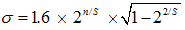
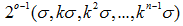
实际计算时,三种方法计算的金字塔组数noctaves,尺度空间坐标σ,以及每组金字塔内的层数S是一样的。同时,假设图像为640*480的标准图像。
金字塔层数:
其中o_min = 0,对于分辨率为640*480的图像N=5。
每组金字塔内图像数:
S=3,即在做极值检测时使用金子塔内中间3张图像。
对于LoG每组金字塔内有S+2张图像(S=-1,0,1,2,3),需要做S+1次高斯模糊操作(后一张图像由前一张做高斯模糊得到);而DoG每组金字塔有S+3张高斯图像,得到S+2张DoG图像。
尺度空间系数:其中,S表示每组金字塔内图像层数,n为当前高斯层数,取0-4。DoG需要5个尺度系数得到6张GSS图像,而LoG只需要前4个尺度系数得到5张图像。
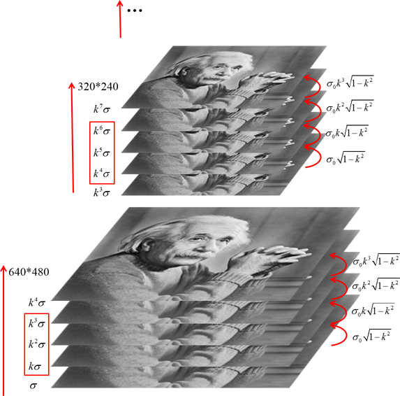
LoG
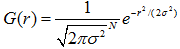
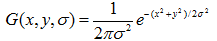
高斯核使用正太分布(高斯函数)计算模糊模版,N维空间正太分布方程为:
于是,二维高斯模板上的距离中心点为(x,y)的元素对应高斯计算公式为:
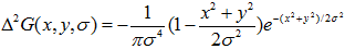
规范化的高斯拉普拉斯图像为
最终构造LoG金字塔有5层,每层有S+2=5张图像,每层金字塔内每张图像尺度是前一张的k倍,即构成的连续尺度序列:
其中o为当前金字塔层数,n为在当前金字塔层中图像张数。
由于卷积计算性质:在计算时,通过对前一张图像做尺度系数为
的卷积操作,可以减少卷积计算次数。故在金字塔每层内的S+2张图像,需要S+1次卷积操作,每次LoG核的尺度系数为:图1. LoG金字塔示意图。 左侧为图像尺度空间系数,红色矩形框为实际参与比较的空间系数,右侧为在上一张图像做LoG卷积操作的尺度系数
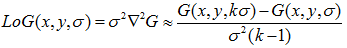
DoG
由于LoG与Gauss核具有如下关系:
即,
因此,LoG算子可以用高斯差分算子DoG(Difference of Guassians)表示。
于是通过高斯金字塔每层内相邻两张图像相减可以得到DoG金字塔。对于最后需要S张图像寻找极值点,需要S+2张DoG图像,S+3张高斯图像。具体关系如图2.所示。
图 2. 由高斯金字塔得到DoG金字塔及其对应的尺度空间系数示意图。
LoG & DoG
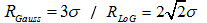
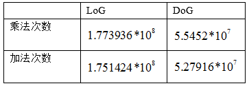
一个直观的比较结果,使用
分别计算LoG和DoG,得到:可以看到,LoG比DoG明显需要更多的加法运算和乘法运算。虽然DoG需要在每层金字塔多做一次高斯操作(即为了得到S+2张DoG图需要S+3张高斯模糊图),但通过减法取代LoG核的计算过程,显著减少了运算次数,大大节省了运算时间。


发布者:全栈程序员-站长,转载请注明出处:https://javaforall.net/181937.html原文链接:https://javaforall.net


