Sklearn中的CV与KFold详解

大家好，又见面了，我是你们的朋友全栈君。如果您正在找激活码,请点击查看最新教程,关注关注公众号 “全栈程序员社区” 获取激活教程,可能之前旧版本教程已经失效.最新Idea2022.1教程亲测有效,一键激活。

Jetbrains全系列IDE使用 1年只要46元售后保障童叟无欺

关于交叉验证,我在之前的文章中已经进行了简单的介绍,而现在我们则通过几个更加详尽的例子.详细的介绍

CV

%matplotlib inline
import numpy as np
from sklearn.model_selection import train_test_split
from sklearn import datasets
from sklearn import svm

iris = datasets.load_iris()
iris.data.shape,iris.target.shape

((150, 4), (150,))

一般的分割方式,训练集-测试集.然而这种方式并不是很好

X_train, X_test, y_train, y_test = train_test_split(iris.data, iris.target, test_size=0.4, random_state=0) 

clf_svc = svm.SVC(kernel='linear').fit(X_train,y_train)
clf_svc.score(X_test,y_test)

0.9666666666666667

缺点一:浪费数据
缺点二:容易过拟合,且矫正方式不方便

这时,我们需要使用另外一种分割方式-交叉验证

from sklearn.model_selection import cross_val_score
clf_svc_cv = svm.SVC(kernel='linear',C=1)
scores_clf_svc_cv = cross_val_score(clf_svc_cv,iris.data,iris.target,cv=5)
print(scores_clf_svc_cv)
print("Accuracy: %0.2f (+/- %0.2f)" % (scores_clf_svc_cv.mean(), scores_clf_svc_cv.std() * 2))

[ 0.96666667  1.          0.96666667  0.96666667  1.        ]
Accuracy: 0.98 (+/- 0.03)

同时我们也可以为cross_val_score选择不同的性能度量函数

from sklearn import metrics
scores_clf_svc_cv_f1 = cross_val_score(clf_svc_cv,iris.data,iris.target,cv=5,scoring='f1_macro')
print("F1: %0.2f (+/- %0.2f)" % (scores_clf_svc_cv_f1.mean(), scores_clf_svc_cv_f1.std() * 2))

F1: 0.98 (+/- 0.03)

同时也正是这些特性使得,cv与数据转化以及pipline(sklearn中的管道机制)变得更加契合

from sklearn import preprocessing
from sklearn.pipeline import make_pipeline
clf_pipline = make_pipeline(preprocessing.StandardScaler(),svm.SVC(C=1))
scores_pipline_cv = cross_val_score(clf_pipline,iris.data,iris.target,cv=5)
print("Accuracy: %0.2f (+/- %0.2f)" % (scores_clf_svc_cv_f1.mean(), scores_clf_svc_cv_f1.std() * 2))

Accuracy: 0.98 (+/- 0.03)

同时我们还可以在交叉验证使用多个度量函数

from sklearn.model_selection import cross_validate
from sklearn import metrics

scoring = ['precision_macro', 'recall_macro']
clf_cvs = svm.SVC(kernel='linear', C=1, random_state=0)
scores_cvs = cross_validate(clf_cvs,iris.data,iris.target,cv=5,scoring=scoring,return_train_score = False)
sorted(scores_cvs.keys())

['fit_time', 'score_time', 'test_precision_macro', 'test_recall_macro']

print(scores_cvs['test_recall_macro'])
print("test_recall_macro: %0.2f (+/- %0.2f)" % (scores_cvs['test_recall_macro'].mean(), scores_cvs['test_recall_macro'].std() * 2))

[ 0.96666667  1.          0.96666667  0.96666667  1.        ]
test_recall_macro: 0.98 (+/- 0.03)

同时cross_validate也可以使用make_scorer自定义度量功能
或者使用单一独量

from sklearn.metrics.scorer import make_scorer
scoring_new = { 
   'prec_macro': 'precision_macro','recall_micro': make_scorer(metrics.recall_score, average='macro')}
# 注意此处的make_scorer
scores_cvs_new = cross_validate(clf_cvs,iris.data,iris.target,cv=5,scoring=scoring_new,return_train_score = False)
sorted(scores_cvs_new.keys())

['fit_time', 'score_time', 'test_prec_macro', 'test_recall_micro']

print(scores_cvs_new['test_recall_micro'])
print("test_recall_micro: %0.2f (+/- %0.2f)" % (scores_cvs_new['test_recall_micro'].mean(), scores_cvs_new['test_recall_micro'].std() * 2))

[ 0.96666667  1.          0.96666667  0.96666667  1.        ]
test_recall_micro: 0.98 (+/- 0.03)

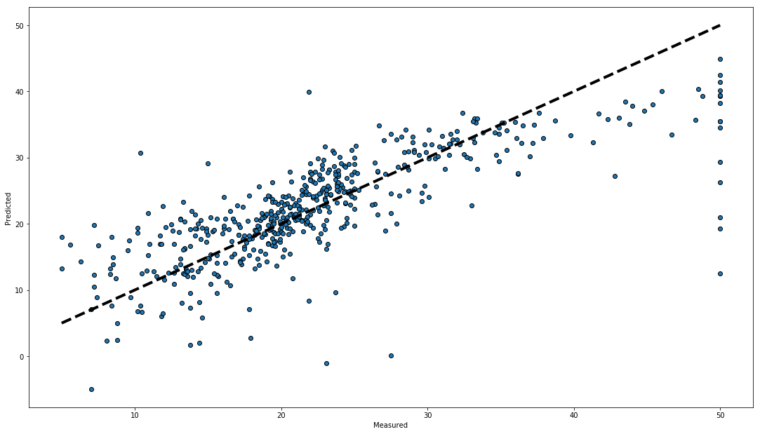
关于Sklearn中的CV还有cross_val_predict可用于预测,下面则是Sklearn中一个关于使用该方法进行可视化预测错误的案例

from sklearn import datasets
from sklearn.model_selection import cross_val_predict
from sklearn import linear_model
import matplotlib.pyplot as plt

lr = linear_model.LinearRegression()
boston = datasets.load_boston()
y = boston.target

# cross_val_predict returns an array of the same size as `y` where each entry
# is a prediction obtained by cross validation:
predicted = cross_val_predict(lr, boston.data, y, cv=10)

fig, ax = plt.subplots()
fig.set_size_inches(18.5,10.5)
ax.scatter(y, predicted, edgecolors=(0, 0, 0))
ax.plot([y.min(), y.max()], [y.min(), y.max()], 'k--', lw=4)
ax.set_xlabel('Measured')
ax.set_ylabel('Predicted')
plt.show()

通过交叉验证进行数据错误的可视化

KFlod的例子

Stratified k-fold:实现了分层交叉切分

from sklearn.model_selection import StratifiedKFold
X = np.array([[1, 2, 3, 4],
              [11, 12, 13, 14],
              [21, 22, 23, 24],
              [31, 32, 33, 34],
              [41, 42, 43, 44],
              [51, 52, 53, 54],
              [61, 62, 63, 64],
              [71, 72, 73, 74]])

y = np.array([1, 1, 0, 0, 1, 1, 0, 0])

stratified_folder = StratifiedKFold(n_splits=4, random_state=0, shuffle=False)
for train_index, test_index in stratified_folder.split(X, y):
    print("Stratified Train Index:", train_index)
    print("Stratified Test Index:", test_index)
    print("Stratified y_train:", y[train_index])
    print("Stratified y_test:", y[test_index],'\n')

Stratified Train Index: [1 3 4 5 6 7]
Stratified Test Index: [0 2]
Stratified y_train: [1 0 1 1 0 0]
Stratified y_test: [1 0] 

Stratified Train Index: [0 2 4 5 6 7]
Stratified Test Index: [1 3]
Stratified y_train: [1 0 1 1 0 0]
Stratified y_test: [1 0] 

Stratified Train Index: [0 1 2 3 5 7]
Stratified Test Index: [4 6]
Stratified y_train: [1 1 0 0 1 0]
Stratified y_test: [1 0] 

Stratified Train Index: [0 1 2 3 4 6]
Stratified Test Index: [5 7]
Stratified y_train: [1 1 0 0 1 0]
Stratified y_test: [1 0]

from sklearn.model_selection import StratifiedKFold
X = np.array([[1, 2, 3, 4],
              [11, 12, 13, 14],
              [21, 22, 23, 24],
              [31, 32, 33, 34],
              [41, 42, 43, 44],
              [51, 52, 53, 54],
              [61, 62, 63, 64],
              [71, 72, 73, 74]])

y = np.array([1, 1, 0, 0, 1, 1, 0, 0])

stratified_folder = StratifiedKFold(n_splits=4, random_state=0, shuffle=False)
for train_index, test_index in stratified_folder.split(X, y):
    print("Stratified Train Index:", train_index)
    print("Stratified Test Index:", test_index)
    print("Stratified y_train:", y[train_index])
    print("Stratified y_test:", y[test_index],'\n')

Stratified Train Index: [1 3 4 5 6 7]
Stratified Test Index: [0 2]
Stratified y_train: [1 0 1 1 0 0]
Stratified y_test: [1 0] 

Stratified Train Index: [0 2 4 5 6 7]
Stratified Test Index: [1 3]
Stratified y_train: [1 0 1 1 0 0]
Stratified y_test: [1 0] 

Stratified Train Index: [0 1 2 3 5 7]
Stratified Test Index: [4 6]
Stratified y_train: [1 1 0 0 1 0]
Stratified y_test: [1 0] 

Stratified Train Index: [0 1 2 3 4 6]
Stratified Test Index: [5 7]
Stratified y_train: [1 1 0 0 1 0]
Stratified y_test: [1 0]

除了这几种交叉切分KFlod外,还有很多其他的分割方式,比如StratifiedShuffleSplit重复分层KFold,实现了每个K中各类别的比例与原数据集大致一致,而RepeatedStratifiedKFold 可用于在每次重复中用不同的随机化重复分层 K-Fold n 次。至此基本的KFlod在Sklearn中都实现了

注意

i.i.d 数据是机器学习理论中的一个常见假设，在实践中很少成立。如果知道样本是使用时间相关的过程生成的，则使用 time-series aware cross-validation scheme 更安全。同样，如果我们知道生成过程具有 group structure （群体结构）（从不同 subjects（主体）， experiments（实验）， measurement devices （测量设备）收集的样本），则使用 group-wise cross-validation 更安全。

下面就是一个分组KFold的例子,

from sklearn.model_selection import GroupKFold

X = [0.1, 0.2, 2.2, 2.4, 2.3, 4.55, 5.8, 8.8, 9, 10]
y = ["a", "b", "b", "b", "c", "c", "c", "d", "d", "d"]
groups = [1, 1, 1, 2, 2, 2, 3, 3, 3, 3]

gkf = GroupKFold(n_splits=3)
for train, test in gkf.split(X, y, groups=groups):
    print("%s %s" % (train, test))

[0 1 2 3 4 5] [6 7 8 9]
[0 1 2 6 7 8 9] [3 4 5]
[3 4 5 6 7 8 9] [0 1 2]

更多内容请参考:sklearn相应手册

发布者：全栈程序员-站长，转载请注明出处：https://javaforall.net/191284.html原文链接：https://javaforall.net

CV

KFlod的例子

相关推荐

JavaScript中window.open（）和Window Location href的区别「建议收藏」

voliate关键字的作用[通俗易懂]

jenkins自动触发构建_触发器定时删除

jdk和jvm区别_java中集合和数组的区别

django的drf框架的优点_一个类要具有可序列化

【QGIS入门实战精品教程】2.1：初识QGIS软件[通俗易懂]

发表回复