
一、ECMWF(方正附近,46,128.75,张志浩)
from netCDF4 import Dataset from netCDF4 import num2date nc_obj = Dataset ( "download.nc" ) # 查看nc文件中的变量 print ( nc_obj.variables.keys() ) odict_keys(['longitude', 'latitude', 'time', 'u10', 'v10', 't2m', 'sp']) # 查看每个变量的单位 for i in nc_obj.variables.keys (): print ( nc_obj.variables[i].units ) degrees_east degrees_north hours since 1900-01-01 00:00:00.0 m s-1 m s-1 K Pa # 查看每个变量的形状(维度) for i in nc_obj.variables.keys (): print ( nc_obj.variables[i].shape ) (21,) (41,) (144,) (144, 41, 21) (144, 41, 21) (144, 41, 21) (144, 41, 21) #取出时间 time=nc_obj['time'][:] print(time[:5]) [ ] #将时间转化为人类可读时间 datetime.datetime time1=num2date(time,units=nc_obj['time'].units) print(time1[:5]) [datetime.datetime(2019, 12, 1, 0, 0) datetime.datetime(2019, 12, 1, 1, 0) datetime.datetime(2019, 12, 1, 2, 0) datetime.datetime(2019, 12, 1, 3, 0) datetime.datetime(2019, 12, 1, 4, 0)] #经度 128.5 14 128.75 15 longitude=nc_obj['longitude'][:] print(longitude) # print(nc_obj['longitude'][14]) [125. 125.25 125.5 125.75 126. 126.25 126.5 126.75 127. 127.25 127.5 127.75 128. 128.25 128.5 128.75 129. 129.25 129.5 129.75 130. ] #纬度 45.5 18 46 16 latitude=nc_obj['latitude'][:] print(latitude) # print(nc_obj['latitude'][18]) # print(nc_obj['latitude'][16]) [50. 49.75 49.5 49.25 49. 48.75 48.5 48.25 48. 47.75 47.5 47.25 47. 46.75 46.5 46.25 46. 45.75 45.5 45.25 45. 44.75 44.5 44.25 44. 43.75 43.5 43.25 43. 42.75 42.5 42.25 42. 41.75 41.5 41.25 41. 40.75 40.5 40.25 40. ] #取出变量blh 10 metre V wind component(10米V风分量) v10=nc_obj['v10'][:] #取出北纬46东经128.75的v10数值 a = [0]*144 for i in range(144): a[i]=nc_obj.variables['v10'][i][16][15] #取出变量10 metre U wind component,(10米U风分量) u10=nc_obj['u10'][:] #取出北纬46东经128.75的u10数值 b = [0]*144 for i in range(144): b[i]=nc_obj.variables['u10'][i][16][15] #对v10和u10平方和开平方 c = [0]*144 for i in range(144): c[i]=(a[i]2+b[i]2)0.5 import matplotlib.pyplot as plt import pandas as pd plt.rc('font', family='SimHei', size=15) #绘图中的中文显示问题,图表字体为SimHei,字号为15 #plt.rcParams['font.sans-serif']=['SimHei'] #用来正常显示中文标签 plt.rcParams['axes.unicode_minus']=False #用来正常显示负号 plt.figure(figsize=(31,8)) plt.title('ECMWF风速(v10和u10平方和的开平方)与时间的函数') #有标题(风速与风向的函数) plt.xlabel('时间') #横坐标的标题 plt.ylabel('风速(m/s)') #纵坐标的标题 plt.grid(color='#95a5a6',linestyle='--',linewidth=3,axis='both',alpha=0.4) #设置网格 plt.plot(time1,c,marker='o',c='r') # plt.xticks(pd.date_range('2019-12-01','2019-01-31')) # plt.xticks(rotation='vertical') # plt.xticks(rotation=30) plt.gcf().autofmt_xdate() # plt.savefig('ECMWF.png') #保存图片 plt.show() D:\Users\zzh\Anaconda3\lib\site-packages\pandas\plotting\_matplotlib\converter.py:103: FutureWarning: Using an implicitly registered datetime converter for a matplotlib plotting method. The converter was registered by pandas on import. Future versions of pandas will require you to explicitly register matplotlib converters. To register the converters: >>> from pandas.plotting import register_matplotlib_converters >>> register_matplotlib_converters() warnings.warn(msg, FutureWarning) 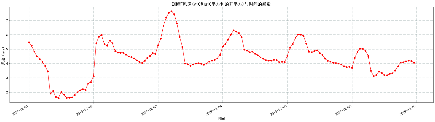

t2m=nc_obj['t2m'][:] # print(t2m) #取出北纬46东经128.75的t2m数值 t2m1 = [0]*144 for i in range(144): t2m1[i]=nc_obj.variables['t2m'][i][16][15] # 将开氏度转化为摄氏度 # 1摄氏度(℃)=274.15开氏度(K) t2m2=[] for i in t2m1: t2m2.append(i/274.15) plt.figure(figsize=(31,8)) plt.title('ECMWF的2米温度(t2m)与时间的函数') #有标题(风速与风向的函数) plt.xlabel('时间') #横坐标的标题 plt.ylabel('温度(K)') #纵坐标的标题 plt.grid(color='#95a5a6',linestyle='--',linewidth=3,axis='both',alpha=0.4) #设置网格 plt.plot(time1,t2m2,marker='o',c='r') # plt.xticks(pd.date_range('2019-12-01','2019-01-31')) # plt.xticks(rotation='vertical') # plt.xticks(rotation=30) plt.gcf().autofmt_xdate() # plt.savefig('ECMWF.png') #保存图片 plt.show() 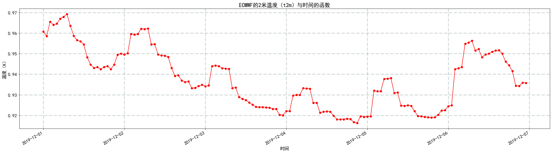
sp=nc_obj['sp'][:] # print(sp) #取出北纬46东经128.75的sp数值 e = [0]*144 for i in range(144): e[i]=nc_obj.variables['sp'][i][16][15] plt.figure(figsize=(31,8)) plt.title('ECMWF的表明压力(sp)与时间的函数') #有标题(风速与风向的函数) plt.xlabel('时间') #横坐标的标题 plt.ylabel('压力(Pa)') #纵坐标的标题 plt.grid(color='#95a5a6',linestyle='--',linewidth=3,axis='both',alpha=0.4) #设置网格 plt.plot(time1,e,marker='o',c='r') # plt.xticks(pd.date_range('2019-12-01','2019-01-31')) # plt.xticks(rotation='vertical') # plt.xticks(rotation=30) plt.gcf().autofmt_xdate() # plt.savefig('ECMWF.png') #保存图片 plt.show() 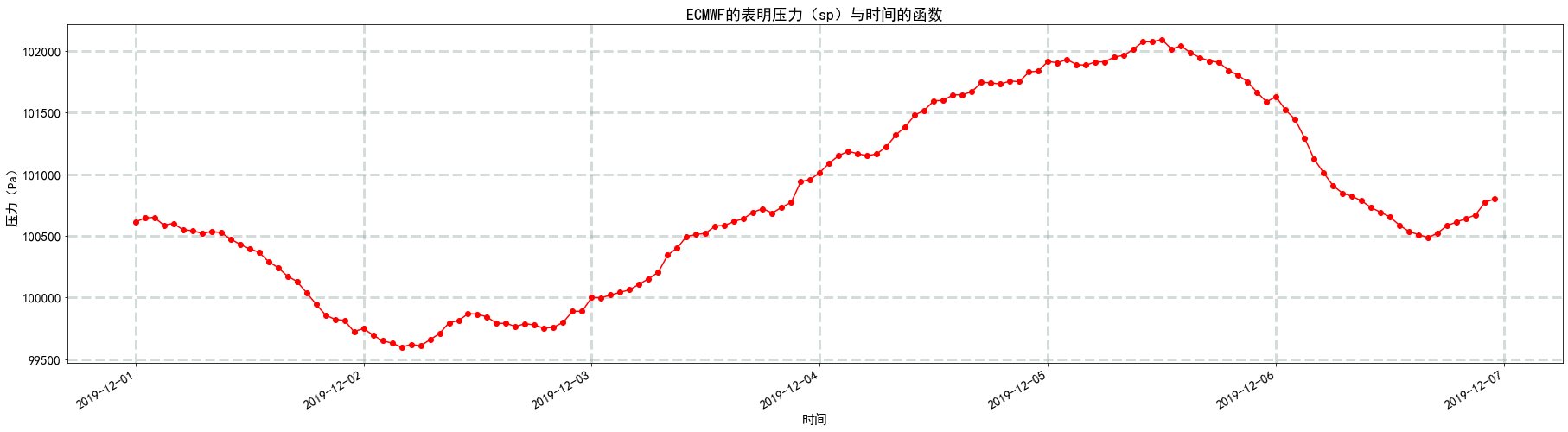
#将数据存储到csv文件 import pandas as pd #a和b的长c度必须保持一致,否则报错 #字典中的key值即为csv中列名 dataframe = pd.DataFrame({
   '时间':time1,'风速(m/s)':c,'2米温度(℃)':t2m2,'压力(Pa)':e}) #将DataFrame存储为csv,index表示是否显示行名,default=True dataframe.to_csv(r"ECMWF(方正)-06.csv",sep=',',index=False)
二、NOAA(通河,45.967 ,128.733王阔)
from datetime import datetime import pandas as pd noaa=pd.read_csv("C:\\Users\\zzh\\Desktop\\tonghe1201-1208.csv") print(noaa.shape) (64, 33) noaa.head() | USAF | WBAN | TIME | DIR | SPD | GUS | CLG | SKC | L | M | … | SLP | ALT | STP | MAX | MIN | PCP01 | PCP06 | PCP24 | PCPXX | SD | |
|---|---|---|---|---|---|---|---|---|---|---|---|---|---|---|---|---|---|---|---|---|---|
| 0 | * | 0 | 261 | 18 | 28 | * | * | * | * | … | 1023.6 | * | 1009.2 | * | * | * | * | 0.19 | * | 0 | |
| 1 | * | 0 | 272 | 12 | 28 | * | * | * | * | … | 1023.4 | * | 1009.0 | * | * | * | 0.00 | 0.19 | * | 0 | |
| 2 | * | 0 | 292 | 7 | 28 | * | * | * | * | … | 1022.7 | * | 1008.3 | 20 | 14 | * | 0.01 | 0.19 | * | 0 | |
| 3 | * | 0 | 300 | 4 | 28 | 722 | CLR | * | * | … | 1022.5 | * | 1007.9 | * | * | * | 0.00 | 0.16 | 0.01 | ||
| 4 | * | 0 | 223 | 1 | 25 | 722 | CLR | * | * | … | 1021.6 | * | 1006.8 | * | * | * | * | 0.05 | * | 0 |
5 rows × 33 columns
#取出时间 TIME=noaa['TIME'][:64,] print(TIME) 0 0 1 0 2 0 3 0 4 0 ... 59 0 60 0 61 0 62 0 63 0 Name: TIME, Length: 64, dtype: int64 # 0, # 每一个时间如上所示,为2019-01-04,15:00 # 我把分钟数截断,因为所有数据分钟数都是00 TIME1=[] for i in TIME: # 0 TIME1.append((str.split(str(i)[:10]))[0]) print(TIME1) ['', '', '', '', '', '', '', '', '', '', '', '', '', '', '', '', '', '', '', '', '', '', '', '', '', '', '', '', '', '', '', '', '', '', '', '', '', '', '', '', '', '', '', '', '', '', '', '', '', '', '', '', '', '', '', '', '', '', '', '', '', '', '', ''] TIME2 =[] for i in TIME1: # TIME2.append(datetime.strptime(i,'%Y%m%d%H')) # # 隔行选取数据 # TIME3 =[] # for i in range(0,247,2): # TIME3 .append(TIME2[i]) SPD=noaa['SPD'][:64,] # print(DIR) #将英里每小时转化为米每秒 # 1英里每小时(mile/h)=0.44704米每秒(m/s) SPD1=[] for i in SPD: SPD1.append(i*0.44704) # print(spd) # # 隔行选取数据 # SPD2 =[] # for i in range(0,247,2): # SPD2 .append(SPD1[i]) plt.figure(figsize=(31,8)) plt.title('NOAA风速与时间的函数') #有标题(风速与风向的函数) plt.xlabel('时间') #横坐标的标题 plt.ylabel('风速(m/s)') #纵坐标的标题 plt.grid(color='#95a5a6',linestyle='--',linewidth=3,axis='both',alpha=0.4) #设置网格 plt.plot(TIME2,SPD1,marker='o',c='g') # plt.xticks(pd.date_range('2019-01-01','2019-01-31')) # plt.xticks(rotation='vertical') # plt.xticks(rotation=30) plt.gcf().autofmt_xdate() # plt.savefig('NOAA.png') #保存图片 plt.show() 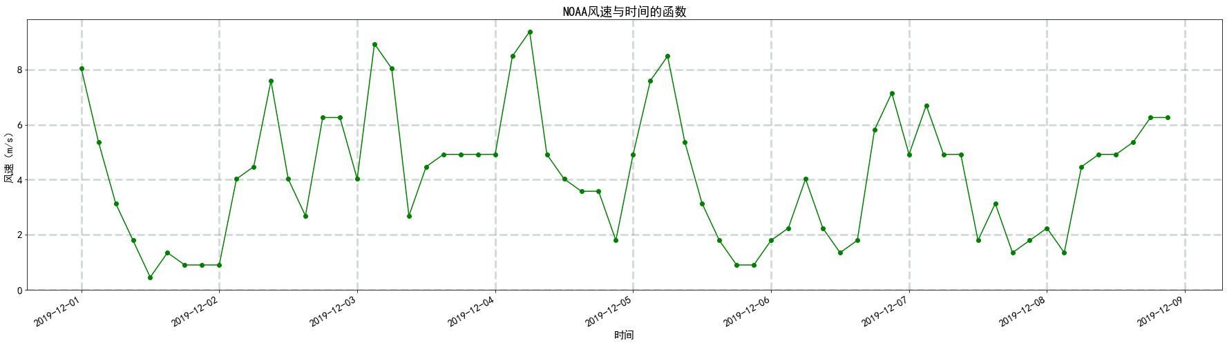
# TEMP 温度 华氏度 TEMP=noaa['TEMP'][:64,] # 将华氏度转化为摄氏度 # 1摄氏度(℃)=33.8华氏度(℉) TEMP1=[] for i in TEMP: TEMP1.append(i/33.8) plt.figure(figsize=(31,8)) plt.title('NOAA温度与时间的函数') #有标题(风速与风向的函数) plt.xlabel('时间') #横坐标的标题 plt.ylabel('温度(℃)') #纵坐标的标题 plt.grid(color='#95a5a6',linestyle='--',linewidth=3,axis='both',alpha=0.4) #设置网格 plt.plot(TIME2,TEMP1,marker='o',c='g') # plt.xticks(pd.date_range('2019-01-01','2019-01-31')) # plt.xticks(rotation='vertical') # plt.xticks(rotation=30) plt.gcf().autofmt_xdate() # plt.savefig('NOAA.png') #保存图片 plt.show() 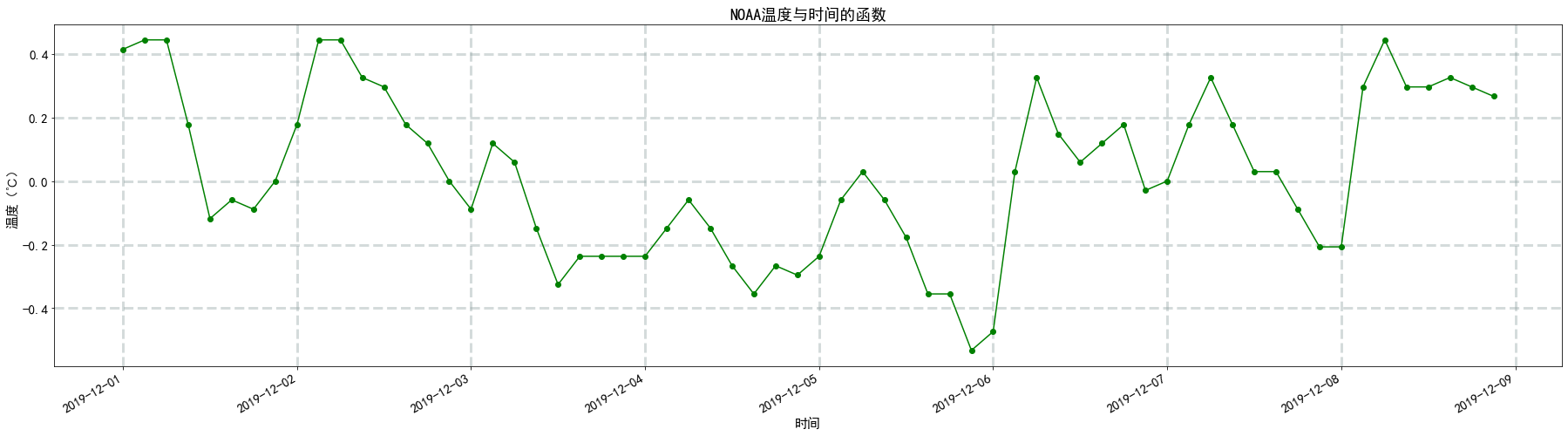
plt.figure(figsize=(31,8)) plt.title('NOAA温度与时间的函数') #有标题(风速与风向的函数) plt.xlabel('时间') #横坐标的标题 plt.ylabel('温度(℃)') #纵坐标的标题 plt.grid(color='#95a5a6',linestyle='--',linewidth=3,axis='both',alpha=0.4) #设置网格 plt.plot(TIME2,TEMP1,marker='o',c='g') # plt.xticks(pd.date_range('2019-01-01','2019-01-31')) # plt.xticks(rotation='vertical') # plt.xticks(rotation=30) plt.gcf().autofmt_xdate() # plt.savefig('NOAA.png') #保存图片 plt.show() 
# STP 站压 毫巴 STP=noaa['STP'][:64,] # 讲毫巴转化成帕 # 1毫巴(mbar)=100帕斯卡(Pa)Pa STP1=[] for i in STP: STP1.append(i*100) plt.figure(figsize=(31,8)) plt.title('NOAA站压与时间的函数') #有标题(风速与风向的函数) plt.xlabel('时间') #横坐标的标题 plt.ylabel('气压(Pa)') #纵坐标的标题 plt.grid(color='#95a5a6',linestyle='--',linewidth=3,axis='both',alpha=0.4) #设置网格 plt.plot(TIME2,STP1,marker='o',c='g') # plt.xticks(pd.date_range('2019-01-01','2019-01-31')) # plt.xticks(rotation='vertical') # plt.xticks(rotation=30) plt.gcf().autofmt_xdate() # plt.savefig('NOAA.png') #保存图片 plt.show() 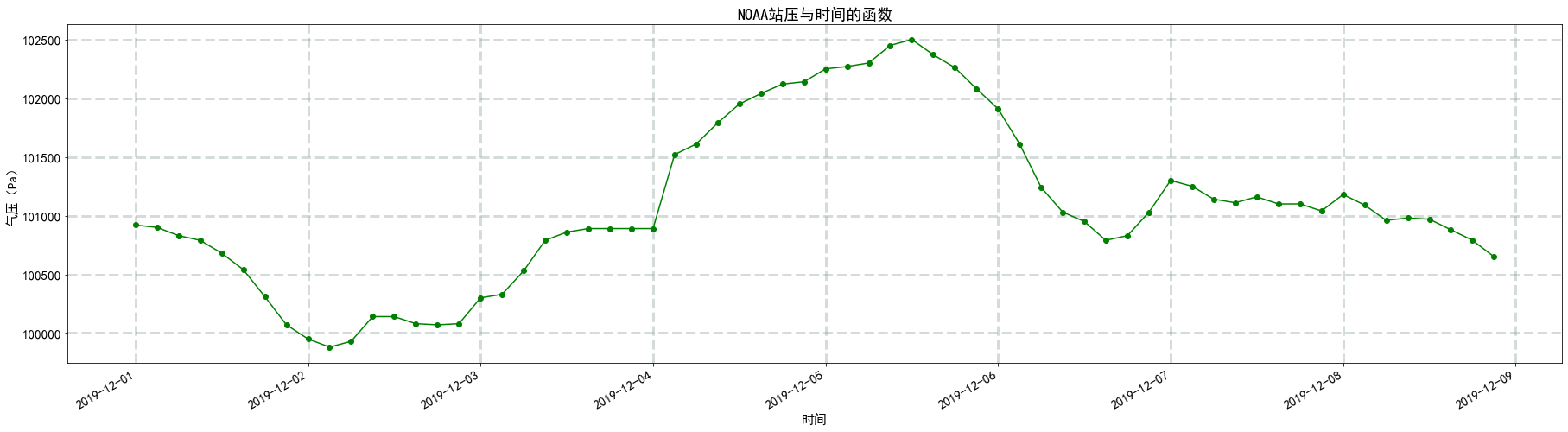
三、中国气象网(方正,45.50,128.48,王阔)
china=pd.read_csv("C:\\Users\\zzh\\Desktop\\方正1202-1208.csv") print(china.head()) Unnamed: 0 Station_Id_C Year Mon Day Hour PRS PRS_Sea PRS_Max \ 0 1 50964 2019 12 2 0 998.4 1014.2 998.5 1 2 50964 2019 12 2 1 998.3 1014.1 998.5 2 3 50964 2019 12 2 2 998.5 1014.3 998.6 3 4 50964 2019 12 2 3 997.8 1013.6 998.5 4 5 50964 2019 12 2 4 997.7 1013.5 997.9 PRS_Min ... WIN_S_Avg_2mi WIN_D_Avg_2mi WEP_Now WIN_S_Inst_Max tigan \ 0 998.3 ... 3.8 206 0.0 8.0 -12.66 1 998.2 ... 2.9 217 22.0 9.6 -12.96 2 998.2 ... 5.8 200 70.0 11.0 -12.70 3 997.8 ... 4.1 220 0.0 11.3 -11.98 4 997.7 ... 5.4 218 70.0 11.9 -12.68 windpower VIS CLO_Cov CLO_Cov_Low CLO_COV_LM 0 3 7200.0 1 3 10500.0 2 3 11200.0 3 3 16900.0 4 3 5000.0 [5 rows x 30 columns] china['Year'] = [str(i) for i in china['Year']] china['Mon'] = [str(i) for i in china['Mon']] china['Day'] = ['0'+str(i) for i in china['Day']] china['Hour'] = [str(i) for i in china['Hour']] # china['time'] = china[['Year', 'Mon','Day','Hour']].apply(lambda x: ''.join(x), axis=1) china['time'] =china['Year']+china['Mon']+china['Day']+china['Hour'] print(china.head()) Unnamed: 0 Station_Id_C Year Mon Day Hour PRS PRS_Sea PRS_Max \ 0 1 50964 2019 12 02 0 998.4 1014.2 998.5 1 2 50964 2019 12 02 1 998.3 1014.1 998.5 2 3 50964 2019 12 02 2 998.5 1014.3 998.6 3 4 50964 2019 12 02 3 997.8 1013.6 998.5 4 5 50964 2019 12 02 4 997.7 1013.5 997.9 PRS_Min ... WIN_D_Avg_2mi WEP_Now WIN_S_Inst_Max tigan windpower \ 0 998.3 ... 206 0.0 8.0 -12.66 3 1 998.2 ... 217 22.0 9.6 -12.96 3 2 998.2 ... 200 70.0 11.0 -12.70 3 3 997.8 ... 220 0.0 11.3 -11.98 3 4 997.7 ... 218 70.0 11.9 -12.68 3 VIS CLO_Cov CLO_Cov_Low CLO_COV_LM time 0 7200.0 1 10500.0 2 11200.0 3 16900.0 4 5000.0 [5 rows x 31 columns] china_time=china['time'] print(china_time) 0 1 2 3 4 ... 163 164 165 166 167 Name: time, Length: 168, dtype: object china_time1 =[] for i in china_time: # china_time1.append(datetime.strptime(i,'%Y%m%d%H')) WIN_S_Avg_2mi=china['WIN_S_Avg_2mi'] plt.figure(figsize=(31,8)) plt.title('中国气象网2分钟平均风速与时间的函数') #有标题(风速与风向的函数) plt.xlabel('时间') #横坐标的标题 plt.ylabel('风速(m/s)') #纵坐标的标题 plt.grid(color='#95a5a6',linestyle='--',linewidth=3,axis='both',alpha=0.4) #设置网格 plt.plot(china_time1,WIN_S_Avg_2mi,marker='o',c='y') # plt.xticks(pd.date_range('2019-01-01','2019-01-31')) # plt.xticks(rotation='vertical') # plt.xticks(rotation=30) plt.gcf().autofmt_xdate() # plt.savefig('NOAA.png') #保存图片 plt.show() 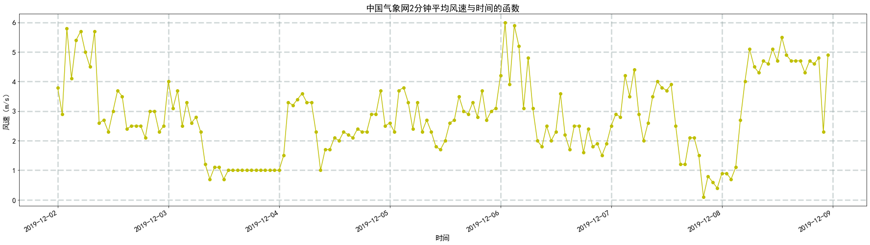
TEM=china['TEM'] # TEM1 = [-i for i in TEM] plt.figure(figsize=(31,8)) plt.title('中国气象网温度与时间的函数') #有标题(风速与风向的函数) plt.xlabel('时间') #横坐标的标题 plt.ylabel('温度(℃)') #纵坐标的标题 plt.grid(color='#95a5a6',linestyle='--',linewidth=3,axis='both',alpha=0.4) #设置网格 plt.plot(china_time1,TEM,marker='o',c='y') # plt.xticks(pd.date_range('2019-01-01','2019-01-31')) # plt.xticks(rotation='vertical') # plt.xticks(rotation=30) plt.gcf().autofmt_xdate() # plt.savefig('NOAA.png') #保存图片 plt.show() 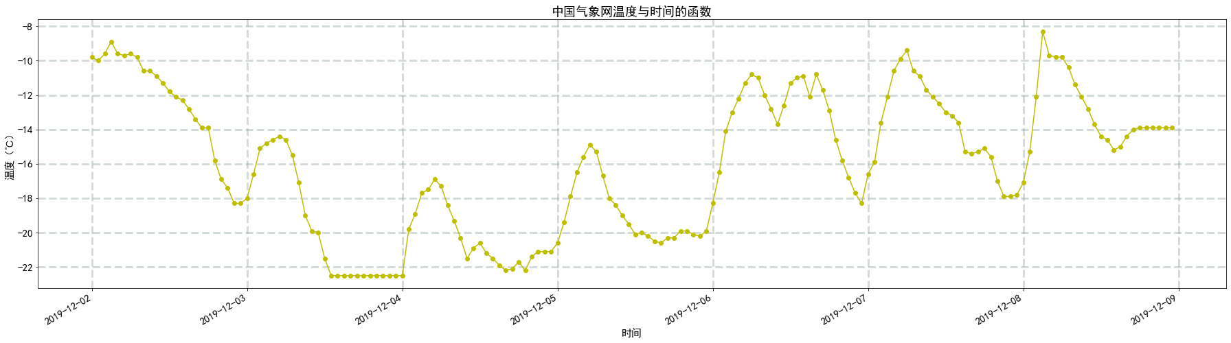
PRS=china['PRS'] # 将百帕转化成帕 # 1百帕(hpa)=100帕斯卡(Pa) PRS1=[] for i in PRS: PRS1.append(i*100) plt.figure(figsize=(31,8)) plt.title('中国气象网气压与时间的函数') #有标题(风速与风向的函数) plt.xlabel('时间') #横坐标的标题 plt.ylabel('气压(Pa)') #纵坐标的标题 plt.grid(color='#95a5a6',linestyle='--',linewidth=3,axis='both',alpha=0.4) #设置网格 plt.plot(china_time1,PRS1,marker='o',c='y') # plt.xticks(pd.date_range('2019-01-01','2019-01-31')) # plt.xticks(rotation='vertical') # plt.xticks(rotation=30) plt.gcf().autofmt_xdate() # plt.savefig('NOAA.png') #保存图片 plt.show() 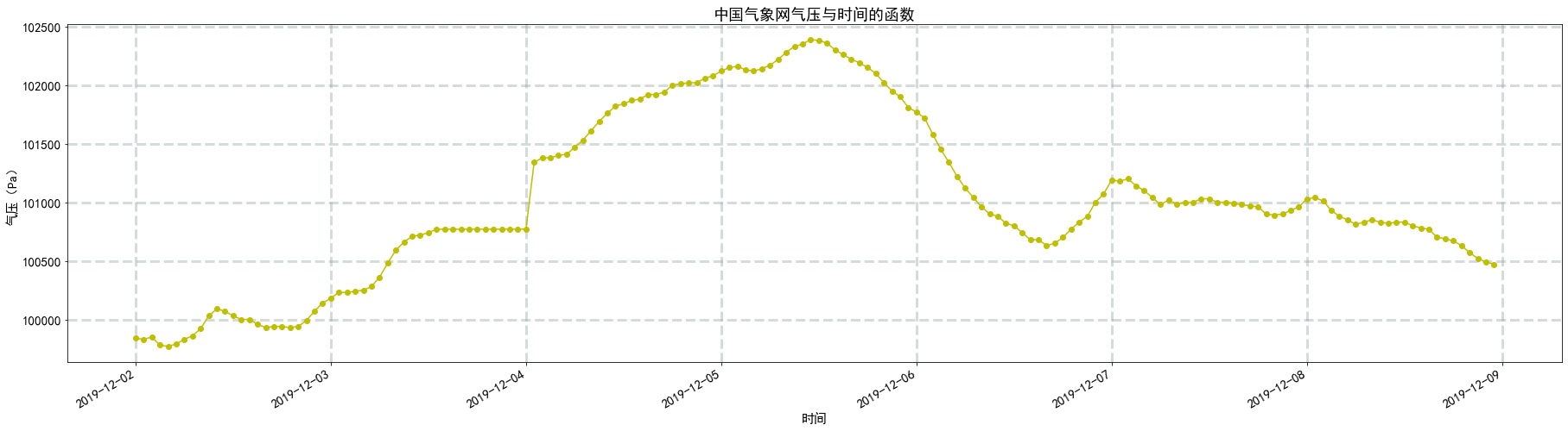
四、GFS(方正附近,46.0、128.75,梁晨)
from datetime import datetime import pandas as pd import matplotlib.pyplot as plt import numpy as np df1 = pd.read_csv("C:\\Users\\zzh\Desktop\\-1209.csv",header=None) print(df1[:5]) 0 1 2 3 4 5 \ 0 2019-12-09 06:00:00 2019-12-09 06:00:00 GUST surface 128.00 45.0 1 2019-12-09 06:00:00 2019-12-09 06:00:00 GUST surface 128.25 45.0 2 2019-12-09 06:00:00 2019-12-09 06:00:00 GUST surface 128.50 45.0 3 2019-12-09 06:00:00 2019-12-09 06:00:00 GUST surface 128.75 45.0 4 2019-12-09 06:00:00 2019-12-09 06:00:00 GUST surface 129.00 45.0 6 0 7.1135 1 2.3135 2 3.2135 3 4.1135 4 3.4135 df1.columns=["time1","time2","WindSpeed","level","longitude","latitude","value"] print(df1[:5]) time1 time2 WindSpeed level longitude \ 0 2019-12-09 06:00:00 2019-12-09 06:00:00 GUST surface 128.00 1 2019-12-09 06:00:00 2019-12-09 06:00:00 GUST surface 128.25 2 2019-12-09 06:00:00 2019-12-09 06:00:00 GUST surface 128.50 3 2019-12-09 06:00:00 2019-12-09 06:00:00 GUST surface 128.75 4 2019-12-09 06:00:00 2019-12-09 06:00:00 GUST surface 129.00 latitude value 0 45.0 7.1135 1 45.0 2.3135 2 45.0 3.2135 3 45.0 4.1135 4 45.0 3.4135 #df2=df1[(df1["longitude"]==128.75)&(df1["latitude"]==46.00)] df1 =df1.sort_values("time1",inplace=False) df1 = df1.reset_index(drop=True) n_time=[] for i in range(0,df1.iloc[:,0].size): if (df1["longitude"][i]==128.75)&(df1["latitude"][i]==46.00): n_time.append(datetime.strptime( df1["time1"][i], "%Y-%m-%d %H:%M:%S")) n_gust=[] for i in range(0,df1.iloc[:,0].size): if (df1["longitude"][i]==128.75)&(df1["latitude"][i]==46.00): n_gust.append(df1["value"][i]) plt.figure(figsize=(30,8)) plt.plot(n_time,n_gust,'go-') plt.title("-09 00:00 06:00 12:00 18:00 GUST") Text(0.5, 1.0, '-09 00:00 06:00 12:00 18:00 GUST') 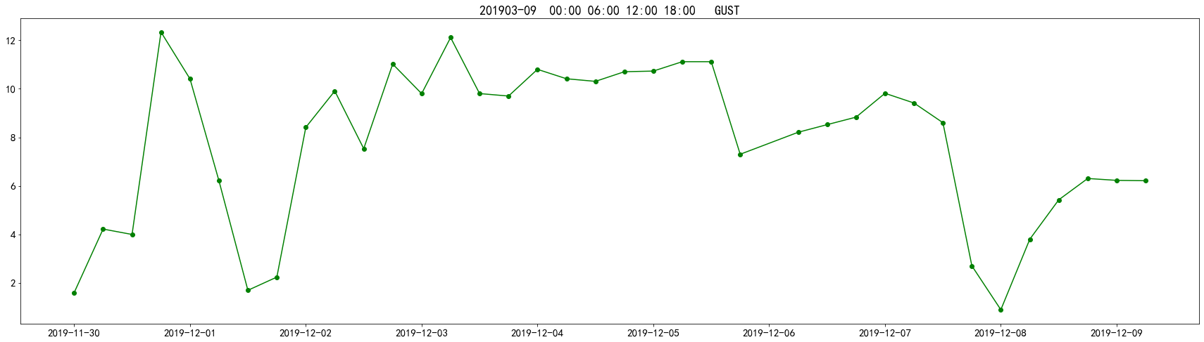
五、对比图
plt.figure(figsize=(31,8)) plt.title('风速与时间的函数') #有标题(风速与风向的函数) plt.xlabel('时间') #横坐标的标题 plt.ylabel('风速(m/s)') #纵坐标的标题 plt.grid(color='#95a5a6',linestyle='--',linewidth=3,axis='both',alpha=0.4) #设置网格 plt.plot(time1,c,marker='o',c='r',label='ECMWF')#ECMWF plt.plot(TIME2,SPD1,marker='o',c='g',label='NOAA')#NOAA plt.plot(n_time,n_gust,marker='o',c='b',label='GFS')#GFS plt.plot(china_time1,WIN_S_Avg_2mi,marker='o',c='y',label='中国气象网')#中国气象网 # plt.xticks(pd.date_range('2019-01-01','2019-01-31')) plt.xticks(rotation='vertical') # plt.xticks(rotation=30) # plt.gcf().autofmt_xdate() plt.legend(loc='best') plt.gcf().autofmt_xdate() plt.savefig('风速对比图') #保存图片 plt.show() 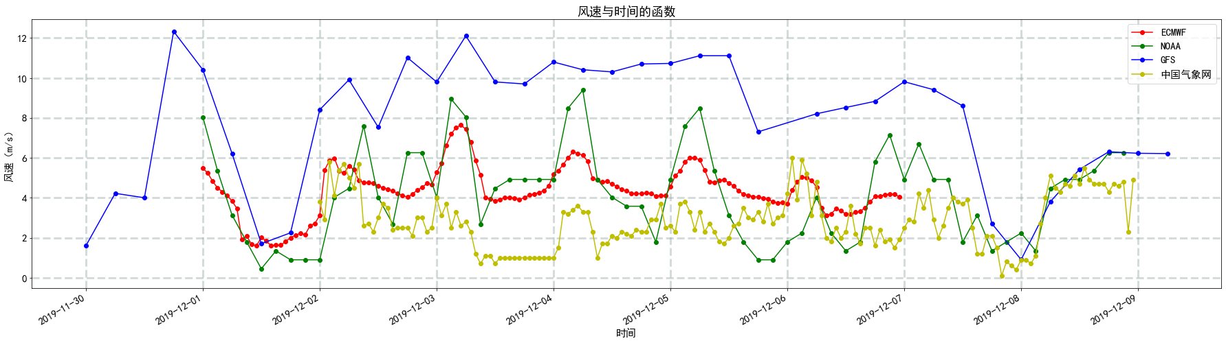
plt.figure(figsize=(31,8)) plt.title('温度与时间的函数') #有标题(风速与风向的函数) plt.xlabel('时间') #横坐标的标题 plt.ylabel('温度(℃)') #纵坐标的标题 plt.grid(color='#95a5a6',linestyle='--',linewidth=3,axis='both',alpha=0.4) #设置网格 plt.plot(time1,t2m2,marker='o',c='r',label='ECMWF')#ECMWF plt.plot(TIME2,TEMP1,marker='o',c='g',label='NOAA')#NOAA # plt.plot(china_time1,TEM,marker='o',c='y',label='中国气象网')#中国气象网 # plt.xticks(pd.date_range('2019-01-01','2019-01-31')) plt.xticks(rotation='vertical') # plt.xticks(rotation=30) # plt.gcf().autofmt_xdate() plt.legend(loc='best') plt.gcf().autofmt_xdate() plt.savefig('温度对比图') #保存图片 plt.show() 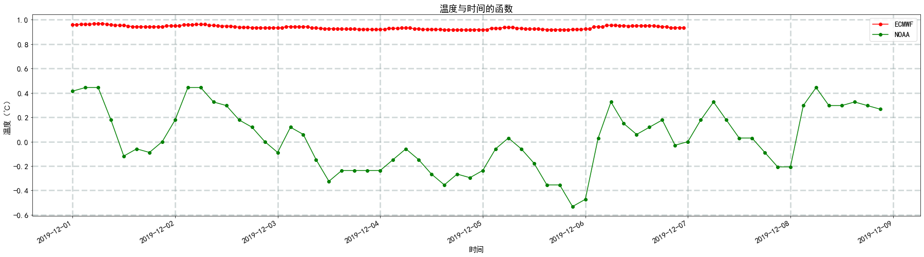
plt.figure(figsize=(31,8)) plt.title('气压与时间的函数') #有标题(风速与风向的函数) plt.xlabel('时间') #横坐标的标题 plt.ylabel('气压(Pa)') #纵坐标的标题 plt.grid(color='#95a5a6',linestyle='--',linewidth=3,axis='both',alpha=0.4) #设置网格 plt.plot(time1,e,marker='o',c='r',label='ECMWF')#ECMWF plt.plot(TIME2,STP1,marker='o',c='g',label='NOAA',)#NOAA plt.plot(china_time1,PRS1,marker='o',c='y',label='中国气象网')#中国气象网 # plt.xticks(pd.date_range('2019-01-01','2019-01-31')) plt.xticks(rotation='vertical') # plt.xticks(rotation=30) # plt.gcf().autofmt_xdate() plt.legend(loc='best') plt.gcf().autofmt_xdate() plt.savefig('气压对比图') #保存图片 plt.show() 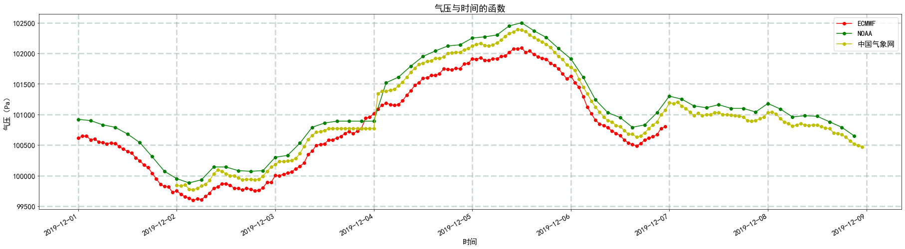
版权声明:本文内容由互联网用户自发贡献,该文观点仅代表作者本人。本站仅提供信息存储空间服务,不拥有所有权,不承担相关法律责任。如发现本站有涉嫌侵权/违法违规的内容, 请联系我们举报,一经查实,本站将立刻删除。
发布者:全栈程序员-站长,转载请注明出处:https://javaforall.net/202683.html原文链接:https://javaforall.net


