一般线性模型和混合线性模型_线性混合模型如何工作

生命科学的数学统计和机器学习 (Mathematical Statistics and Machine Learning for Life Sciences)

This is the seventeenth article from my column Mathematical Statistics and Machine Learning for Life Sciences where I try to explain some mysterious analytical techniques used in Bioinformatics and Computational Biology in a simple way. Linear Mixed Model (LMM) also known as Linear Mixed Effects Model is one of key techniques in traditional Frequentist statistics. Here I will attempt to derive LMM solution from scratch from the Maximum Likelihood principal by optimizing mean and variance parameters of Fixed and Random Effects. However, before diving into derivations, I will start slowly in this post with an introduction of when and how to technically run LMM. I will cover examples of linear modeling from both Frequentist and Bayesian frameworks.

这是我的《生命科学的数学统计和机器学习》专栏中的第十七篇文章，我试图以一种简单的方式来解释生物信息学和计算生物学中使用的一些神秘的分析技术。 线性混合模型(LMM)也称为线性混合效应模型，是传统频率统计中的关键技术之一。 在这里，我将尝试通过优化固定效应和随机效应的均值和方差参数，从最大似然原理从头开始 获得LMM解决方案。 但是，在深入探讨衍生工具之前，我将在本文中慢慢介绍何时以及如何在技术上运行LMM 。 我将介绍来自频繁框架和贝叶斯框架的线性建模示例。

数据非独立性问题 (Problem of Non-Independence in Data)

Traditional Mathematical Statistics is based to a large extent on assumptions of the Maximum Likelihood principal and Normal distribution. In case of e.g. multiple linear regression these assumptions might be violated if there is non-independence in the data. Provided that data is expressed as a p by n matrix, where p is the number of variables and n is the number of observations, there can be two types of non-independence in the data:

传统的数学统计在很大程度上是基于最大似然原理和正态分布的假设 。 在例如多重线性回归的情况下，如果数据中存在非独立性 ，则可能会违反这些假设。 假设数据用ap x n矩阵表示，其中p是变量数，n是观察数，则数据中可以有两种类型的非独立性：

• non-independent variables / features (multicollinearity)

  非独立变量/特征( 多重共线性 )

• non-independent statistical observations (grouping of samples)

  非独立统计观察(样本分组)

In both cases, the inverse data matrix needed for the solution of Linear Model is singular, because its determinant is close to zero due to correlated variables or observations. This problem is particularly manifested when working with a high-dimensional data (p >> n) where variables can become redundant and correlated, this is known as the Curse of Dimensionality.

在这两种情况下，线性模型求解所需的逆数据矩阵都是奇异的 ，因为由于相关变量或观测值，其行列式接近于零。 当使用高维数据(p >> n)时，此问题尤其明显，其中变量可能变得多余且相关，这称为维数诅咒 。

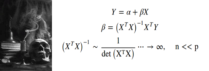
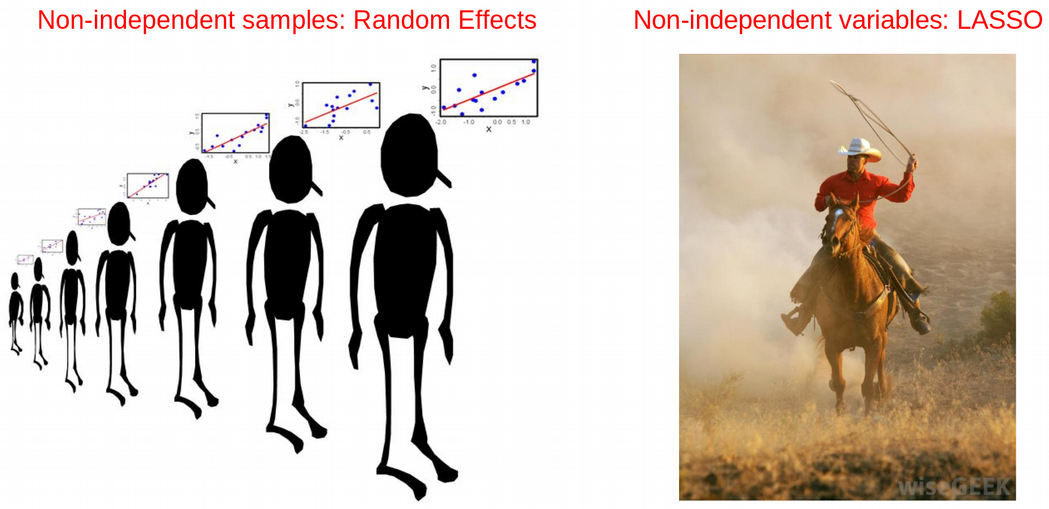
To overcome the problem of non-independent variables, one can for example select most informative variables with LASSO, Ridge or Elastic Net regression, while the non-independence among statistical observations can be taking into account via Random Effects modelling within the Linear Mixed Model.

为了克服非独立变量的问题，例如可以使用LASSO ，Ridge或Elastic Net回归选择最具信息量的变量，而统计观测值之间的非独立性可以通过线性混合模型中的 随机效应建模加以考虑。

I covered a few variable selection methods including LASSO in my post Select Features for OMICs Integration. In the next section, we will see an example of longitudinal data where grouping of data points should be addressed through the Random Effects modelling.

在我的文章《 用于OMIC集成的选择功能》中，我介绍了一些变量选择方法，包括LASSO。 在下一部分中，我们将看到一个纵向数据的示例，其中应通过随机效应建模解决数据点分组的问题。

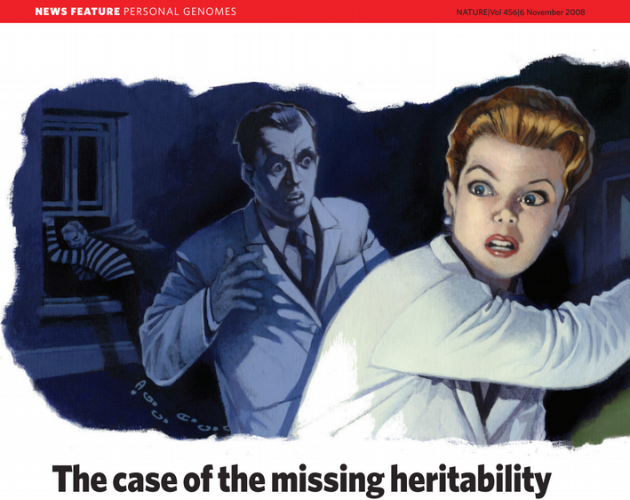
LMM and Random Effects modeling are widely used in various types of data analysis in Life Sciences. One example is the GCTA tool that contributed a lot to the research of long-standing problem of Missing Heritability. The idea of GCTA is to fit genetic variants with small effects all together as Random Effect withing LMM framework. Thanks to the GCTA model the problem of Missing Heritability seems to be solved at least for Human Height.

LMM和随机效应建模广泛用于生命科学中的各种类型的数据分析。 GCTA工具就是一个例子，它为长期遗留 遗传力问题的研究做出了很大贡献。 GCTA的想法是将具有较小影响的遗传变异体与具有LMM框架的随机效应结合在一起。 多亏了GCTA模型，遗传力缺失的问题似乎至少对于人类身高可以解决 。

Another popular example from computational biology is the Differential Gene Expression analysis with DESeq / DESeq2R package that does not really run LMM but performs a variance stabilization/shrinkage that is one of essential points of LMM. The advantage of this approach is that lowly expressed genes can borrow some information from the highly expressed genes that allows for their more stable and robust testing.

来自计算生物学的另一个流行示例是使用DESeq / DESeq2 R软件包进行的差异基因表达分析， 该软件包不能真正运行LMM，但可以执行方差稳定化 /收缩，这是LMM的关键点之一。 这种方法的优势在于，低表达的基因可以从高表达的基因中借用一些信息，从而可以进行更稳定，更可靠的测试。

Finally, LMM is one of the most popular analytical techniques in Evolutionary Science and Ecology where they use the state-of-the-art MCMCglmm package for estimating e.g. trait heritability.

最后，LMM是进化科学和生态学中最流行的分析技术之一，它们使用最先进的MCMCglmm软件包来估计例如性状遗传力 。

数据非独立性的示例 (Example of Non-Independence in Data)

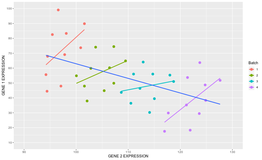
As we concluded previously, LMM should be used when there is some sort of clustering among statistical observations / samples. This can be, for example, due to different geographic locations where the samples were collected, or different experimental protocols that produced the samples. Batch-effects in Biomedical Sciences is an example of such a grouping factor that leads to non-independence between statistical observations. If not properly corrected for, batch-effects in RNAseq data can lead to totally opposite co-expression pattern between two genes (Simpson’s paradox).

正如我们先前得出的结论，当统计观测值/样本之间存在某种聚类时，应使用LMM。 例如，这可能是由于收集样品的地理位置不同或产生样品的实验方案不同所致。 生物医学科学中的批量效应就是这种分组因子的一个例子，这种分组因子导致了统计观察结果之间的独立性。 如果不能正确校正，RNAseq数据中的批处理效应可能导致两个基因之间完全相反的共表达模式( 辛普森悖论 )。

Another example can be a genetic relation between individuals. Finally, this can be repetitive measurements performed on the same individuals but at different time points, i.e. technical (not biological) replicates.

另一个例子可以是个体之间的遗传关系 。 最后，这可以是对同一个人但在不同时间点进行的重复测量 ，即技术(非生物学)重复。

As an example of such clustering, we will consider a sleep deprivation study where sleeping time of 18 individuals was restricted, and a Reaction of their organism on a series of tests was measured during 10 days. The data includes three variables: 1) Reaction, 2) Days, 3) Subject, i.e. the same individual was followed during 10 days. To check how the overall reaction of the individuals changed as a response to the sleep deprivation, we will fit an Ordinary Least Squares (OLS) Linear Regression with Reaction as a response variable and Days as a predictor / explanatory variable with lm and display it with ggplot.

作为此类聚类的一个示例，我们将考虑一项睡眠剥夺研究 ，其中限制了18个人的睡眠时间，并在10天内测量了他们的生物在一系列测试中的React 。 数据包括三个变量：1)React，2)天，3)对象，即在10天内跟踪了同一个人。 为了检查个体的整体React如何随着对睡眠剥夺的React而变化，我们将lm拟合为普通最小二乘(OLS)线性回归，其中React为React变量，天为预测变量/解释变量，并将其显示为ggplot 。

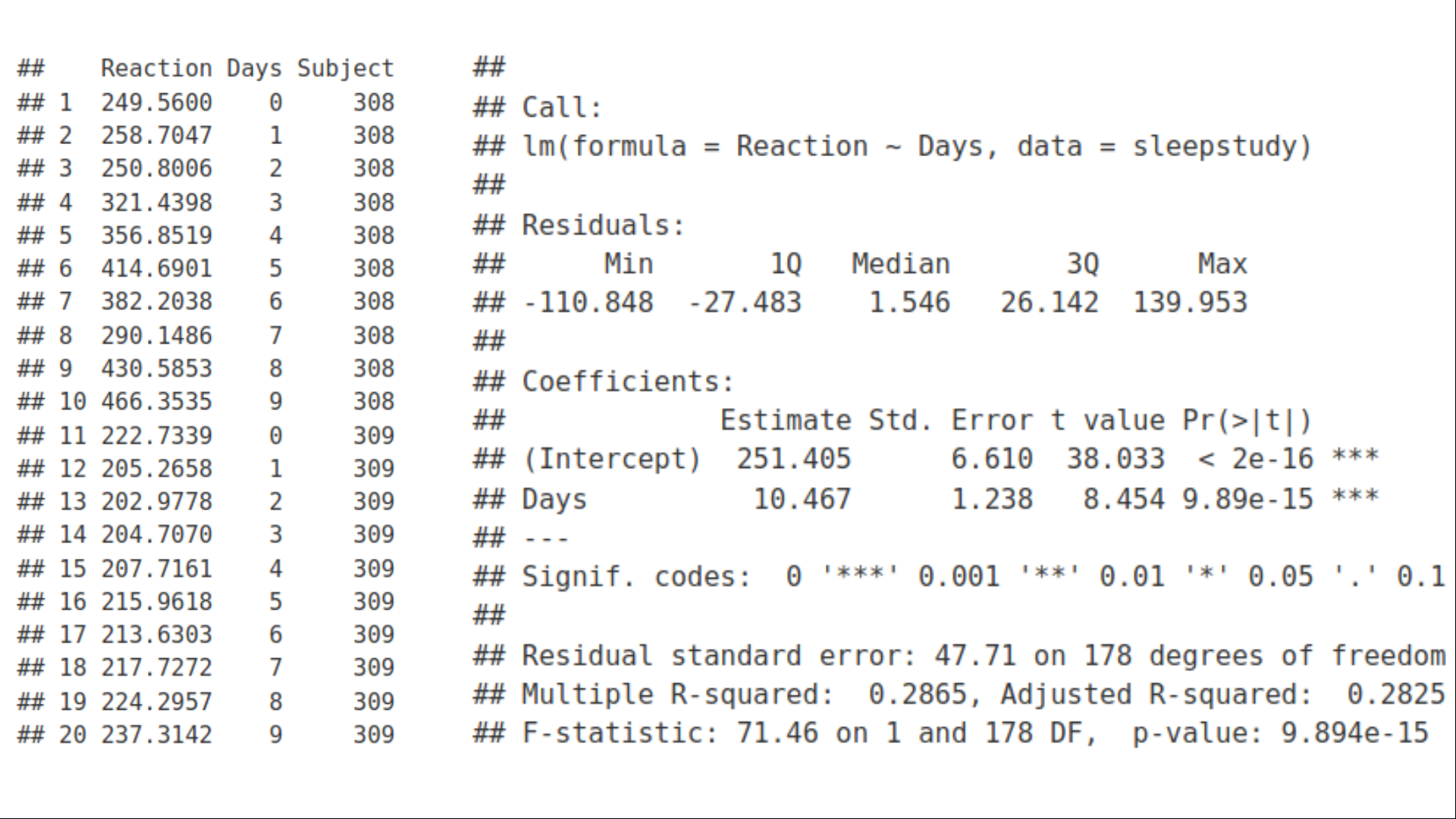
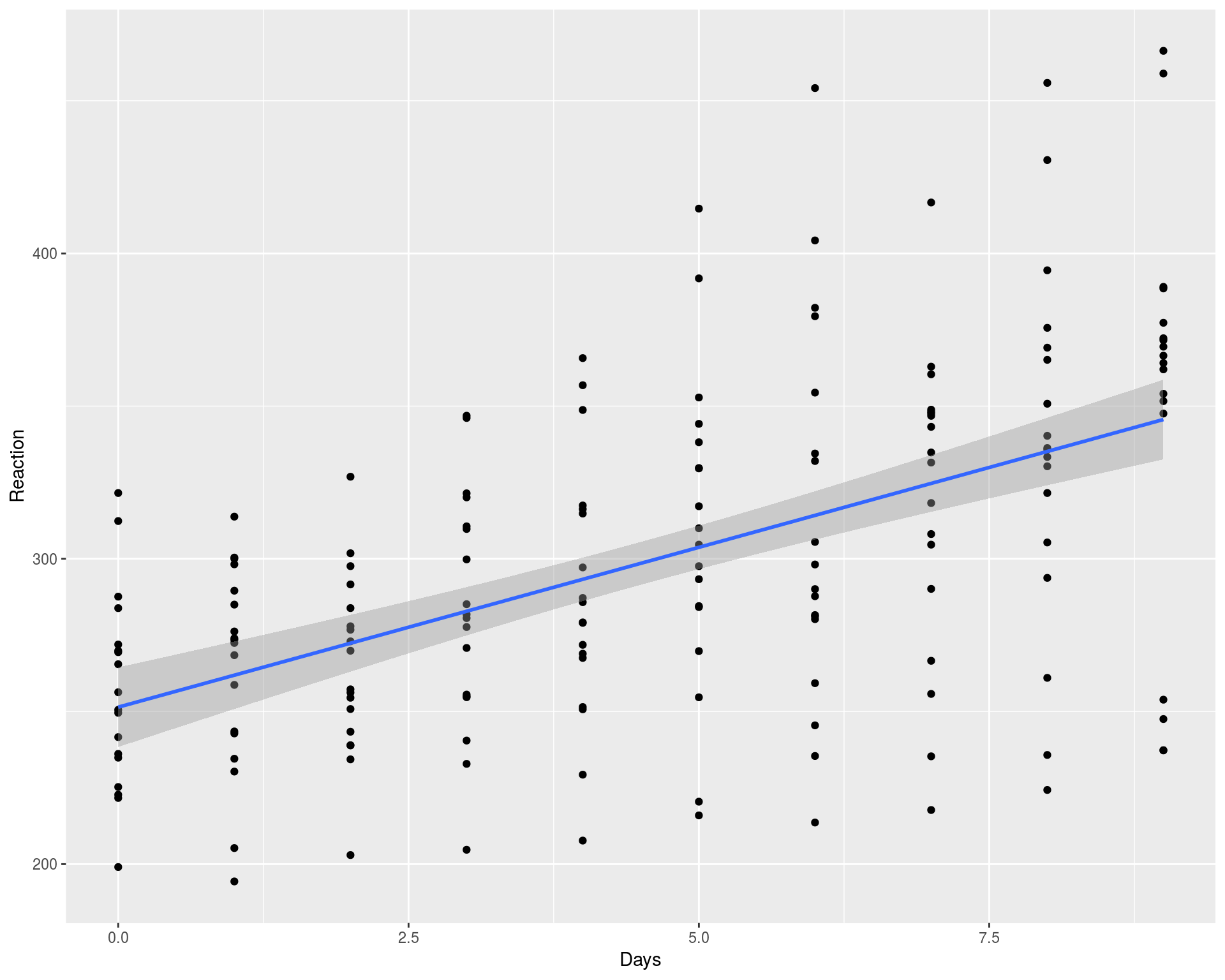
We can observe that Reaction vs. Days has a increasing trend but with a lot of variation between days and individuals. Looking at the summary of the linear regression fit, we conclude that the slope is significantly different from zero, i.e. there is a statistically significant increasing relation between Reaction and Days. The grey area around the fitting line represents 95% confidence interval according to the formula:

我们可以观察到，Respons vs. Days呈上升趋势，但天与个人之间存在很大差异。 查看线性回归拟合的摘要，我们得出结论，斜率与零显着 不同 ，即，“React”和“天”之间存在统计上显着的增加关系。 拟合线周围的灰色区域表示根据公式的95％置信区间：

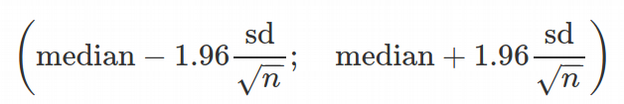
The magic number 1.96 originates from the Gaussian distribution and reflects a Z-score value covering 95% of the data in the distribution. To demonstrate how the confidence intervals are calculated under the hood by ggplot we will implement an identical Linear Regression fit in plain R using predict function.

幻数1.96来自高斯分布，反映的Z分数覆盖分布中95％的数据 。 为了演示如何通过ggplot在引擎盖下计算置信区间，我们将使用预测函数在平原R中实现相同的线性回归拟合。

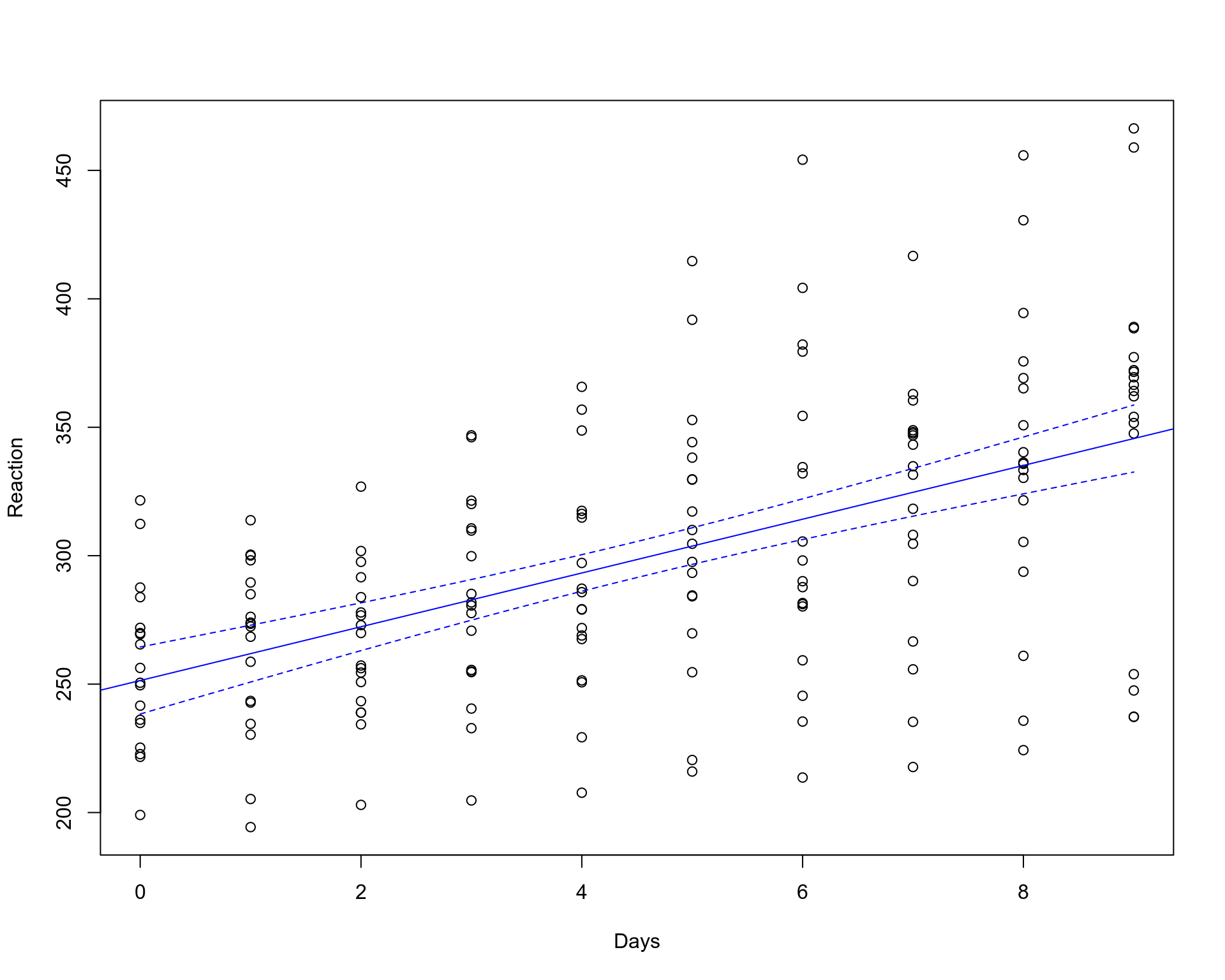
However, there is a problem with the fit above. The Ordinary Least Squares (OLS) assumes that all the observations are independent, which will result in uncorrelated and hence Normally distributed residuals. However, we know that the data points on the plot belong to 18 individuals (10 for each), i.e. the data points cluster within individuals and therefore are not independent. As an alternative way, we can fit linear model (lm) for each individual separately.

但是， 上面的拟合存在问题 。 普通最小二乘(OLS)假设所有观测值都是独立的 ，这将导致不相关且因此呈正态分布的残差 。 但是，我们知道该图上的数据点属于18个个体(每个个体10个)，即，数据点在个体内成簇 ，因此不是独立的 。 作为一种替代方法，我们可以分别拟合每个人的线性模型( lm )。

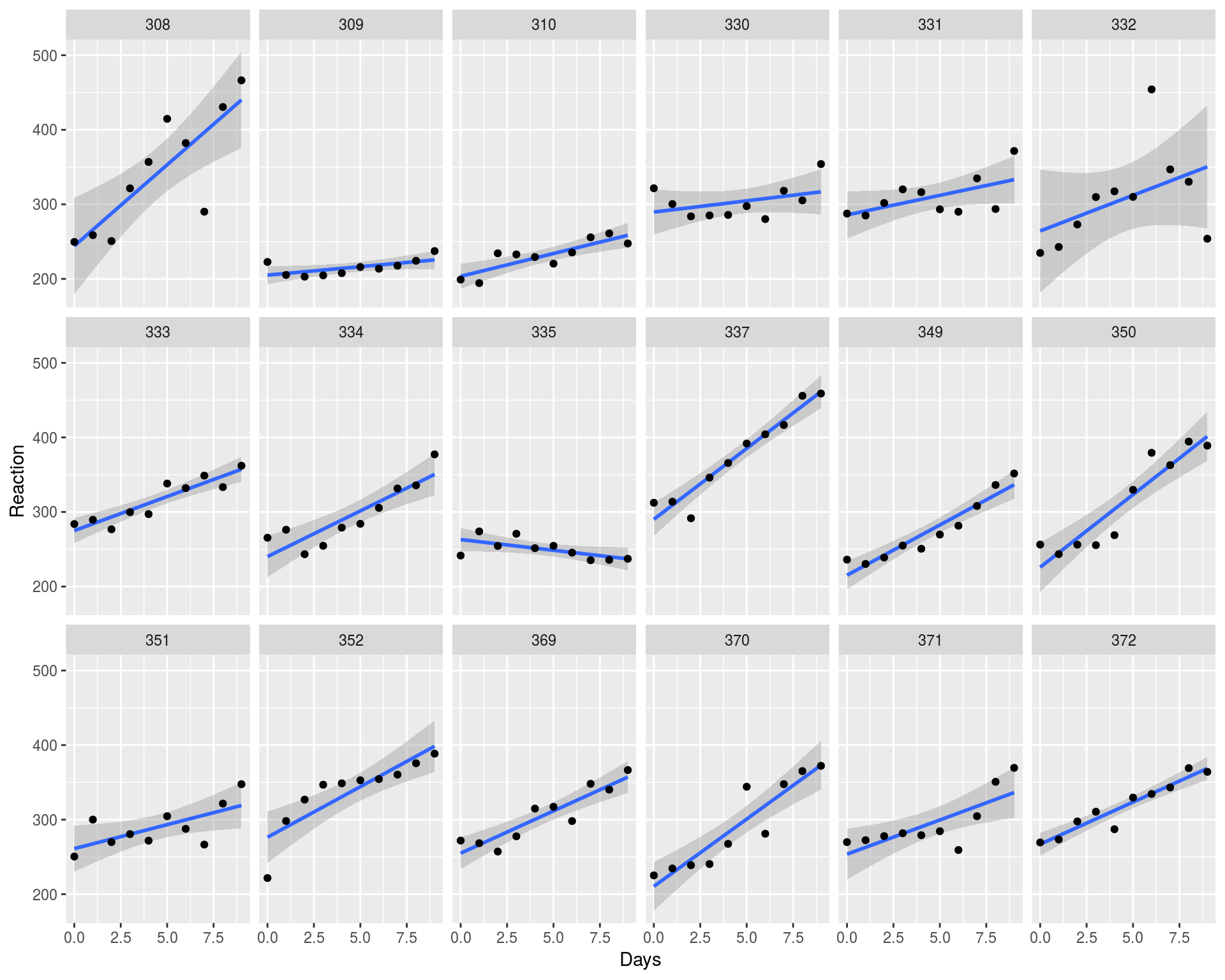
We can see that most of the individuals have increasing Reaction profile while some have a neutral or even decreasing profile. Doesn’t it looks strange that the overall Reaction increases while individual slopes might be decreasing? Is the fit above really good enough?

我们可以看到，大多数人的React曲线都在增加，而有些人则是中性甚至 下降 。 整体React增加而单个斜率可能正在减少，这看起来并不奇怪吗？ 上面的合身真的足够好吗？

Did we capture all the variation in the data with the naive Ordinary Least Squares (OLS) Linear Regression model?

我们是否使用朴素的普通最小二乘(OLS)线性回归模型捕获了数据中的所有变化 ？

The answer is NO because we have not taken the non-independence between data points into account. As we will see later, we can do it much better with a Linear Mixed Model (LMM) that accounts for non-independence between the samples via Random Effects. Despite the term “Random Effects” might sound mysterious, we will show below that it is essentially equivalent to introducing one more fitting parameter in the Maximum Likelihood optimization.

答案是否定的，因为我们没有考虑数据点之间的非独立性。 正如我们将在后面看到的，我们可以使用线性混合模型(LMM)来做得更好，该模型通过随机效应考虑了样本之间的非独立性。 尽管“随机效应”一词听起来似乎很神秘，但我们将在下面显示它基本上等效于在“最大似然性”优化中引入一个更合适的参数 。

频率线性混合模型 (Frequentist Linear Mixed Model)

The naive linear fit that we used above is called Fixed Effects modeling as it fixes the coefficients of the Linear Regression: Slope and Intercept. In contrast Random Effects modeling allows for individual level Slope and Intercept, i.e. the parameters of Linear Regression are no longer fixed but have a variation around their mean values.

我们上面使用的幼稚线性拟合称为固定效果 建模，因为它固定了线性回归的系数：斜率和截距。 相反，“随机效应”建模允许单个级别的“斜率”和“截距”，即线性回归的参数不再固定，而是在其平均值附近有所变化 。

This concept reminds a lot about Bayesian statistics where the parameters of a model are random while the data is fixed, in contrast to Frequentist approach where parameters are fixed but the data is random. Indeed, later we will show that we obtain similar results with both Frequentist Linear Mixed Model and Bayesian Hierarchical Model. Another strength of LMM and Random Effects is that the fit is performed on all individuals simultaneously in the context of each other, that is all individual fits “know” about each other. Therefore, the slopes, intercepts and confidence intervals of the individual fits are affected by their common statistic, shared variance, this is called shrinkage toward the mean, we will cover it in more details when deriving LMM from scratch in the next post.

这个概念使人们想起了很多有关贝叶斯统计的问题 ，其中，在数据固定的情况下模型的参数是随机的，与在参数固定但数据是随机的情况下的频繁性方法相反。 的确，稍后我们将证明，使用“ 频繁线性混合模型”和“ 贝叶斯 层次模型”都可以获得类似的结果。 LMM和随机效应的另一个优势是，在彼此的上下文中同时对所有个体执行拟合，也就是说，所有个体彼此“了解” 。 因此，各个拟合的斜率，截距和置信区间受其共同统计量( 共享方差)影响 ，这被称为“均值收缩” ，在下一篇文章中从零开始导出LMM时，我们将更详细地介绍它。

We will fit LMM with random slopes and intercepts for the effect of Days for each individual (Subject) using lmer function from lme4 R package. This will correspond to adding the (Days | Subject) term to the linear model Reaction ~ Days that was previously used inside the lm function.

我们将使用lme4 R包中的lmer函数，为LMM拟合随机斜率并截取天数对每个个体(对象)的影响。 这将对应于将(Days | Subject)项添加到lm函数之前使用的线性模型Reaction〜Days中。

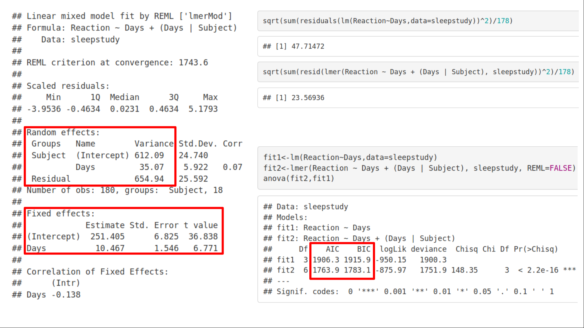
We can immediately see two types of statistics reported: Fixed and Random Effects. The slope and intercept values for Fixed Effects look fairly similar to the ones obtained above with the OLS Linear Regression. On the other hand, the Random Effects statistics is where the adjustment for non-independence between samples occurs. We can see two types of variance reported: the one shared across slopes and intercepts, Name = (Intercept) and Name = Days, that reflects grouping the data points by Subject, and a Residual variance that remains un-modelled, i.e. we can not further reduce this variance within the given model. Further, comparing the Residual errors between Fixed (lm) and Random (lmer) effects models, we can see that the Residual error decreased for the Random Effects model meaning that we captured more variation in the response variable with the Random Effects model. The same conclusion can be drawn from comparing AIC and BICvalues for the two models, again the LMM with Random Effects simply fits the data better. Now let us visualize the difference between Fixed Effects modeling vs. LMM modeling.

我们可以立即看到报告的两种统计信息： 固定效应和随机效应 。 固定效果的斜率和截距值看起来与上面使用OLS线性回归获得的斜率和截距值非常 相似 。 另一方面，“随机效应”统计是在样本之间进行非独立性调整的地方。 我们可以看到报告了两种类型的方差 ：一种是跨坡度和截距共享的 ，即Name =(Intercept)和Name = Days，它反映了按Subject对数据点进行分组，而Residual方差仍未建模，即我们无法在给定模型内进一步减小这种差异。 此外，通过比较固定效应( lm )和随机效应( lmer )模型之间的残差，我们可以看到随机效应模型的残差降低了，这意味着我们用随机效应模型捕获 了响应变量中的更多变化 。 通过比较两个模型的AIC 和 BIC 值可以得出相同的结论，具有随机效应的LMM再次可以更好地拟合数据。 现在让我们可视化固定效果建模与LMM建模之间的区别。

For this reason, we need to visualize confidence intervals of the LMM model. The standard way to build confidence intervals in the Frequentist / Maximum Likelihood framework is via bootstrapping. We will start with the population level (overall / average) fit, and re-run it a number of times using resampling with replacement and randomly removing 75% of samples for each iteration. At each iteration I am going to save LMM fit statistics. After the bootstrapped statistics have been accumulated, I am going to make two plots: first, showing bootstrapped LMM fits against the naive Fixed Effects fit used in the previous section; second, from the accumulated bootstrapped LMM fits I will compute the median, i.e. 50% percentile, as well as 5% and 95% percentiles that will determine the confidence intervals of the population level LMM fit, this will again be plotted versus the naive Fixed Effects fit.

因此，我们需要可视化LMM模型的置信区间 。 在频繁/最大可能性框架中建立置信区间的标准方法是通过引导 。 我们将从总体水平(总体/平均)拟合开始，并使用替换进行重采样并在每次迭代中随机删除75％的样本来重新运行多次。 在每次迭代中，我将保存LMM拟合统计信息。 在累积了自举统计信息之后，我将作两个图：首先，显示自举LMM与上一节中使用的天真的“固定效果”拟合的拟合；以及 第二，从累积的自举LMM拟合中 ，我将计算中位数 ，即50％百分位数，以及将确定总体水平LMM拟合的置信区间的5％和95％百分位数，将再次与朴素的固定值作图效果合适。

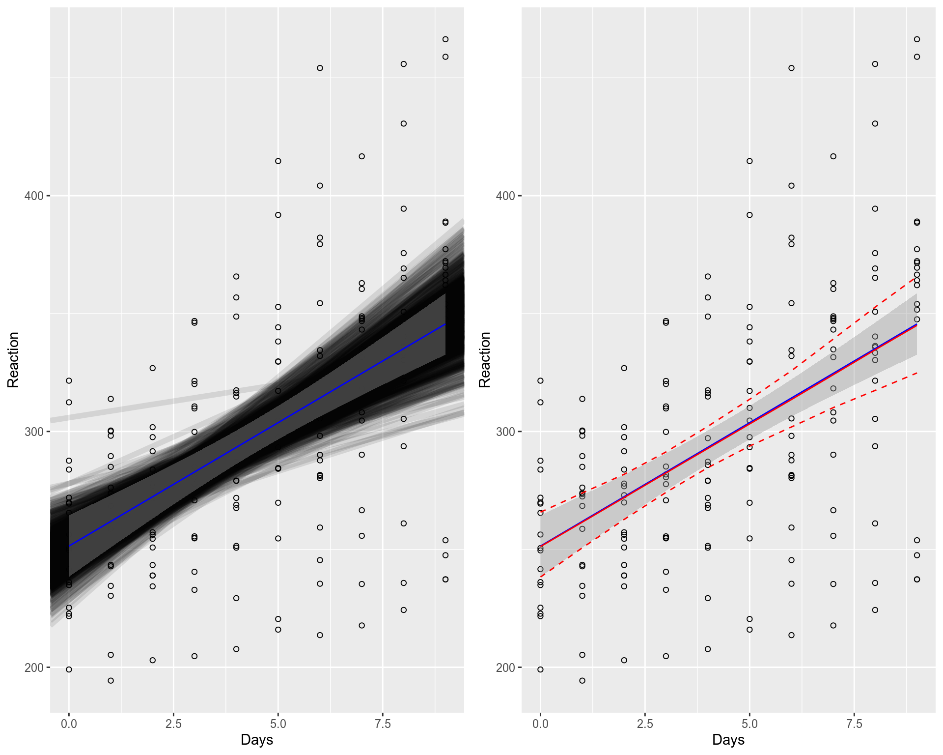
Above, the Fixed Effects fit (blue line + grey 95% confidence intervals area) is displayed together with the computed bootstrapped LMM fits (left plot), and the summary statistics (percentiles) of the bootstrapped LMM fits (right plot). We can observe that the population level LMM fit (lmer, red line, right plot) is very similar to the Fixed Effects fit (lm, blue line on both plots), the difference is hardly noticeable, they overlap well. However, the computed bootstrapped fits (black thick lines, left plot) and confidence intervals for LMM (red dashed line, right plot) are a bit wider than for the Fixed Effects fit (grey area on both plots). This difference is partially due to the fact that the Fixed Effects fit does not account for individual level variation in contrast to LMM that accounts for both population and individual level variations.

上方显示了固定效果拟合(蓝线+ 95％的灰色置信区间灰色区域)以及计算出的自举LMM拟合(左图)和自举LMM拟合的摘要统计量(百分数)(右图)。 我们可以观察到，总体水平的LMM拟合(lmer，红线，右图)与固定效应拟合(两个图上的lm，蓝线)非常相似，差异几乎不明显，它们重叠得很好。 但是，LMM的计算的自举拟合(黑色粗线，左侧图)和置信区间(红色虚线，右侧图)比固定效果拟合(两个图上的灰色区域) 宽一些。 这种差异部分是由于固定效应拟合不考虑个体水平差异，而LMM却同时考虑了人口和个体水平差异。

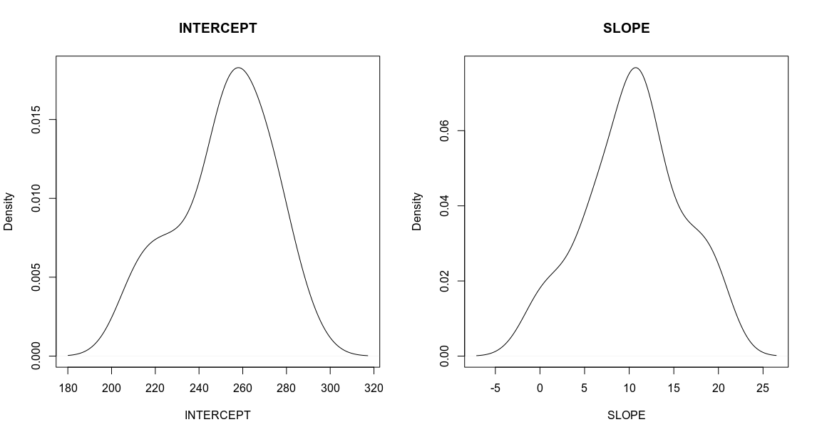
Another interesting thing is that we observe variations of Slope and Intercept around their mean values:

另一个有趣的事情是，我们观察到“斜率”和“截距”均值附近的变化：

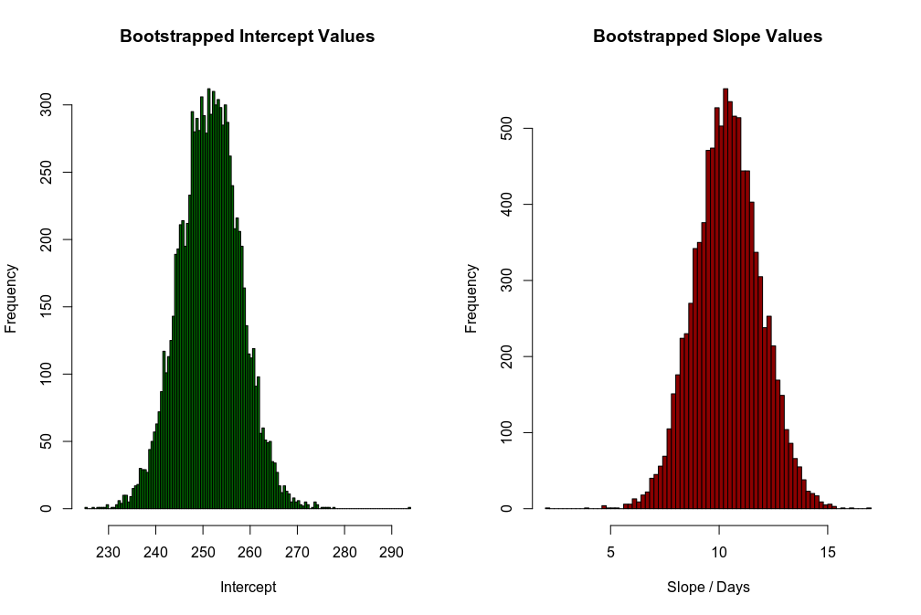
Therefore, one can hypothesize that the bootstrapping procedure for building confidence intervals within Frequentist framework can be viewed as allowing the slopes and intercepts to follow some initial (Prior) distributions, and then sampling their plausible values from the distributions. This sounds much like Bayesian statistics. Indeed, bootstrapping is very similar to the working horse of Bayesian statistics which is Markov Chain Monte Carlo (MCMC). In other words, Frequentist analysis with bootstrapping is to a large extent equivalent to Bayesian analysis, we will revisit this later in more details.

因此，可以假设在Frequentist框架内建立置信区间的引导过程可以看作是允许斜率和截距遵循某些初始( Prior )分布，然后从分布中采样其合理值。 这听起来很像贝叶斯统计。 确实，自举非常类似于贝叶斯统计工作的马可夫链蒙特卡洛(MCMC) 。 换句话说，带有自举的频繁分析在很大程度上等效于贝叶斯分析，我们将在后面更详细地讨论。

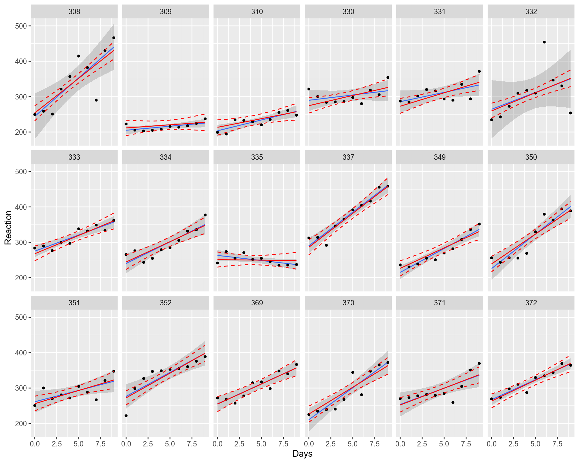
What about individual slopes, intercepts and confidence intervals for each of the 18 individuals from the sleep deprivation study? Here we again plot their Fixed Effects statistics together with the LMM statistics.

睡眠剥夺研究的18个人中每个人的个人斜率，截距和置信区间如何？ 在这里，我们再次绘制其固定效应统计数据和LMM统计数据。

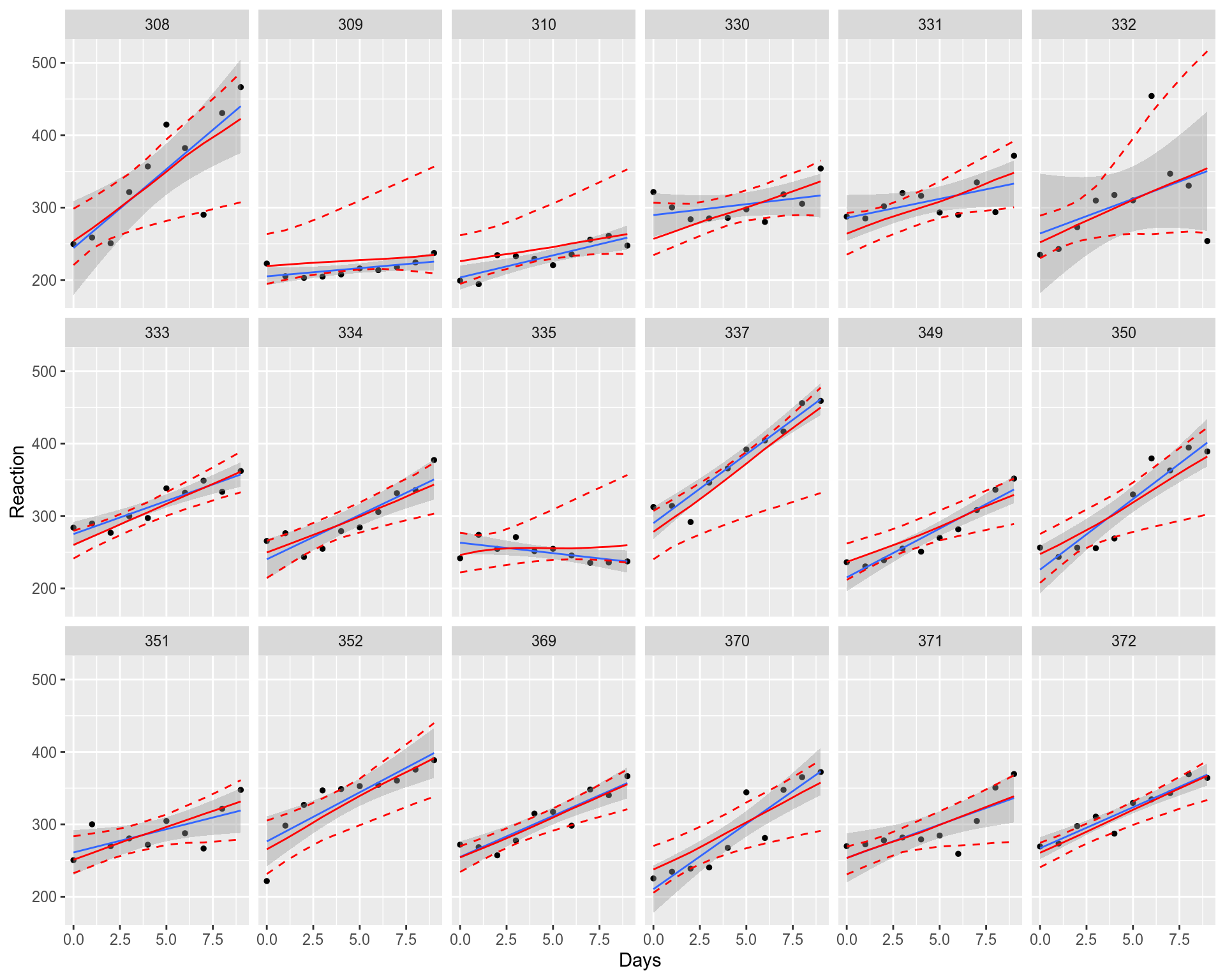
Again, red solid and dashed lines correspond to the LMM fit while blue solid line and the grey area depict Fixed Effects Model. We can see that individual LMM fits (lmer) and their confidence intervals might be very different from the Fixed Effects (lm) model. In other words the individual fits are “shrunk” toward their common population level mean / median, all the fits help each other to have more stable and resembling population level slopes, intercepts and confidence intervals. In the next post, when deriving LMM from scratch, we will understand that this shrinkage toward the mean effect is achieved by adding one more fitting parameter (shared variance) in the Maximum Likelihood optimization procedure.

同样，红色实线和虚线对应于LMM拟合，而蓝色实线和灰色区域则表示固定效果模型。 我们可以看到，单个LMM拟合(lmer)及其置信区间可能与固定效应(lm)模型有很大不同 。 换句话说，个体拟合将“收缩”至其共同的人口水平均值/中位数，所有拟合都相互帮助，从而使人口水平斜率，截距和置信区间更加稳定和相似。 在下一篇文章中，当从零开始推导LMM时，我们将理解，通过在最大似然优化过程中添加一个更多的拟合参数(共享方差)来实现向均值效果的缩小 。

频繁/最大似然与贝叶斯拟合 (Frequentist / Maximum Likelihood vs. Bayesian Fit)

Before moving to the Bayesian Multilevel Models, let us briefly introduce the major differences between Frequentist and Bayesian approaches. Frequentist fit used by LMM through lme4 / lmer is based on the Maximum Likelihood principle, where we maximize the likelihood L(y) of observing the data y, which is equivalent to minimizing residuals of the model, the Ordinary Least Squares approach. In contrast, Bayesian linear model is based on Maximum Posterior Probability principle, where we assume the data to be distributed with some likelihood L(y), and add a Prior assumption on the parameters of the Linear Model.

在转到贝叶斯多级模型之前，让我们简要介绍一下频率和贝叶斯方法之间的主要区别。 LMM通过lme4 / lmer使用的频繁拟合是基于最大似然原理，其中我们将观察数据y的可能性L(y)最大化，这相当于最小化模型的残差(普通最小二乘法)。 相反，贝叶斯线性模型基于最大后验概率原理，在该模型中，我们假设数据以某种似然L(y)分布，并在线性模型的参数上添加了一个先验假设。

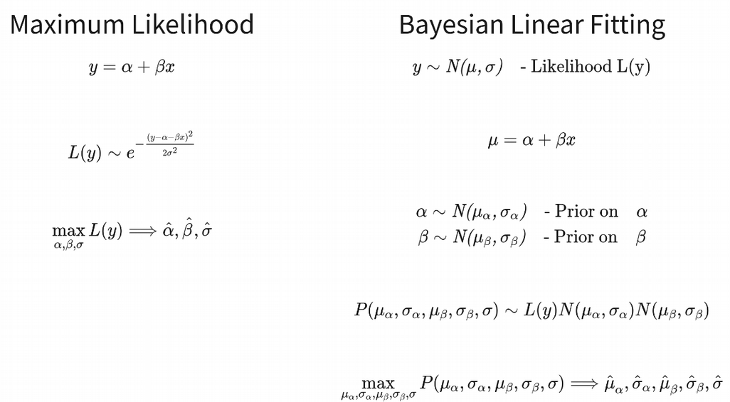
Here we calculate a probability distribution of parameters (and not the data) of the model, which automatically gives us uncertainties (Credible Intervals) on the parameters.

在这里，我们计算模型参数(而不是数据)的概率分布，这将自动为我们提供参数的不确定性(可信区间)。

贝叶斯多层次模型 (Bayesian Multilevel Model)

Linear Mixed Models (LMM) with Bayesian Prior distributions applied to the parameters are called Bayesian Multilevel Models or Bayesian Hierarchical Models. Here, for implementing Bayesian fitting, we will use brms R package that has an identical to lme4 / lmer syntax. However, an important difference to remember is that fitting LMM via lme4 / lmer applies Maximum Likelihood (ML) principle, i.e. it does not use prior assumptions about the parameters (or one case say, it uses flat Priors), while Bayesian Multilevel Model in brms sets reasonable priors reflecting the data. Another thing worth mentioning is that brms uses probabilistic programming language Stan under the hood. We start with Bayesian population level fitting using brms and display the results:

将贝叶斯 先验分布应用于参数的线性混合模型(LMM)称为贝叶斯多级模型或贝叶斯层次模型 。 在这里，为了实现贝叶斯拟合，我们将使用与lme4 / lmer语法相同的brms R包。 但是，要记住的一个重要区别是，通过lme4 / lmer拟合LMM应用了最大似然(ML)原理，即，它不使用关于参数的先验假设(或者说，它使用平坦的先验)，而贝叶斯多级模型用于brms设置反映数据的合理先验。 值得一提的另一件事是， brms在后台使用了概率编程语言Stan 。 我们从使用brms的贝叶斯总体水平拟合开始，并显示结果：

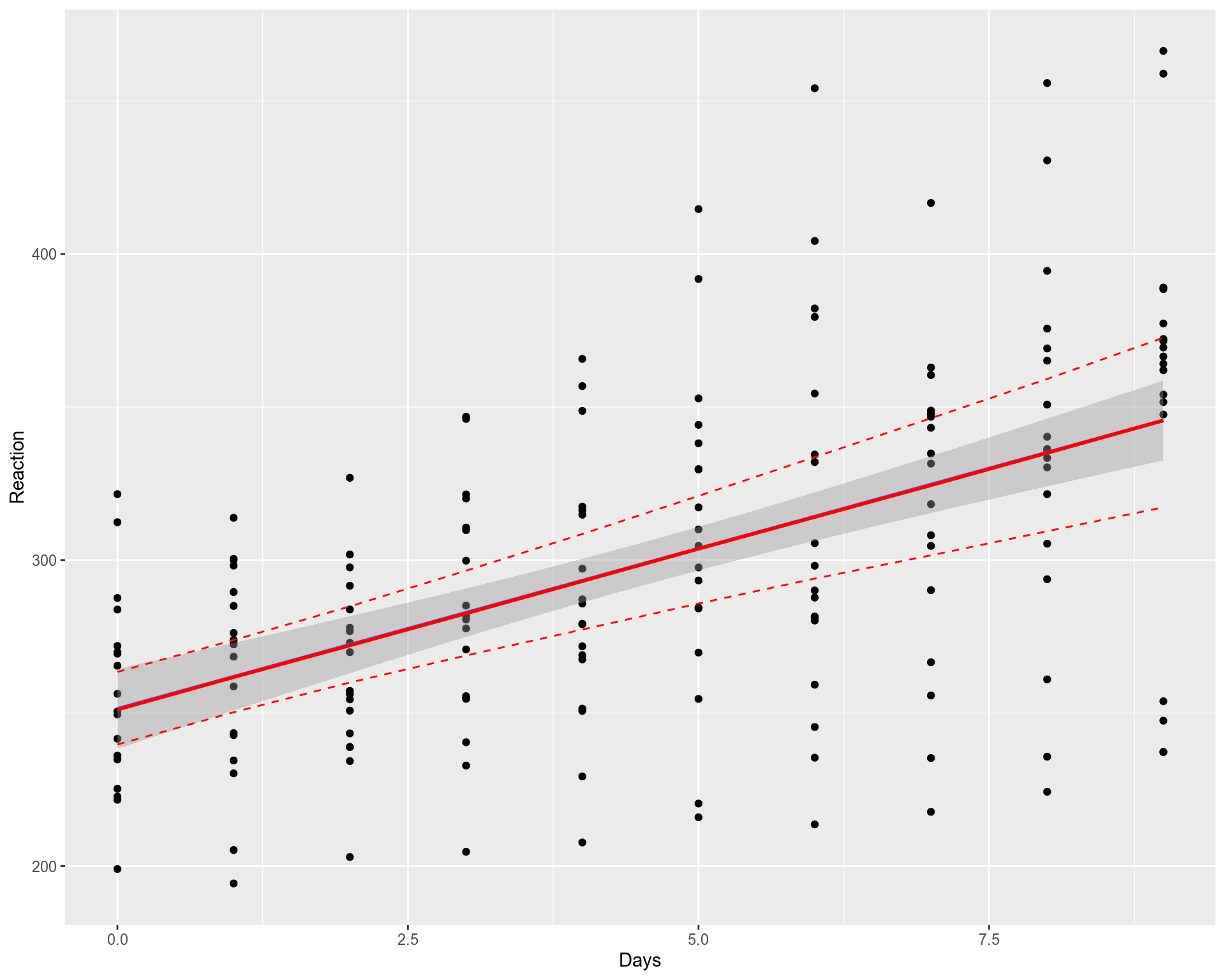
Above, we again plot the Fixed Effects population level fit by the blue line and grey area for confidence intervals, we also add the population level Bayesian Multilevel Model using the solid red line for median and red dashed lines for credible intervals. As for the case of bootstrapped LMM fit, we can conclude that population level Bayesian Multilevel fit perfectly overlaps with the Fixed Effects fit, while the Bayesian credible intervals are somewhat wider than the 95% confidence intervals of the Fixed Effects fit. What about individual fits?

上图，我们再次画出了固定效果人口水平，用置信区间的蓝线和灰色区域拟合，我们还使用实心红色线表示中值，红色虚线表示可信区间 ，添加了人口级别贝叶斯多级模型 。 对于自举LMM拟合，我们可以得出结论：总体水平的贝叶斯多层拟合与固定效应拟合完全重叠 ，而贝叶斯可信区间比固定效应拟合的95％置信区间稍宽 。 那个人适合呢？

Similarly to the individual bootstrapped Frequentist LMM fits, we can see that the individual Bayesian fits with brms (red solid lines) do not always converge to the Fixed Effects Frequentist fits (blue solid lines), but rather “try” to align with the overall population level fit (previous plot) in order to be as similar to each other as possible. The Bayesian credible intervals look again sometimes very different compared to the Frequentist Fixed Effects confidence intervals. This is the result of using Bayesian Priors and accounting for non-normality and non-independence in the data via the multi-level modeling.

类似于各个自举的Frequentist LMM拟合，我们可以看到带有brms的单个Bayes拟合(红色实线)并不总是收敛于Fixed Effects Frequentist拟合(蓝色实线)，而是“尝试”以与总体对齐总体水平拟合(上一个图)，以便彼此尽可能相似 。 与贝叶斯固定效应置信区间相比，贝叶斯可信区间有时有时看起来也非常不同 。 这是使用贝叶斯先验并通过多级建模解决数据中非正常性和非独立性的结果。

摘要 (Summary)

In this post, we have learnt that the Frequentist Linear Mixed Model (LMM) and Bayesian Multilevel (Hierarchical) Model are used to account for non-independence and hence non-normality of data points. The models usually provide a better fit and explain more variation in the data compared to the Ordinary Least Squares (OLS) linear regression model (Fixed Effect). While the population level mean fit of the models typically converges to the Fixed Effect model, the individual fits as well as credible and confidence intervals can be very different reflecting better accounting for non-normality in data.

在这篇文章中，我们了解到，频繁线性混合模型(LMM)和贝叶斯多层次(分层)模型用于说明数据点的非独立性和非正态性。 与普通最小二乘(OLS)线性回归模型(固定效应)相比，该模型通常可提供更好的拟合度并解释数据的更多变化 。 尽管模型的总体水平均值拟合通常收敛于固定效应模型，但个体拟合以及可信度和置信区间可以非常不同，这反映了对数据非正态性的更好解释。

In the comments below, let me know which analytical techniques from Life Sciences seem especially mysterious to you and I will try to cover them in the future posts. Check the codes from the post on my Github. Follow me at Medium Nikolay Oskolkov, in Twitter @NikolayOskolkov and do connect in Linkedin. In the next post, we are going to derive the Linear Mixed Model and program it from scratch from the Maximum Likelihood, stay tuned.

在下面的评论中，让我知道生命科学的哪些分析技术对您来说似乎特别神秘 ，我将在以后的文章中尝试介绍它们。 在我的Github上检查帖子中的代码。 跟随我在中型Nikolay Oskolkov，在Twitter @NikolayOskolkov上进行连接，并在Linkedin中进行连接。 在下一篇文章中，我们将导出线性混合模型，并从“最大似然”中重新编程 ，敬请期待。