时序数据预测：ARIMA

本文尝试应用ARIMA时间序列模型对具有明显季节规律的月度时序数据进行预测，样本数据来源于本人项目工作中的某地区某行业电量（已脱敏处理），外加搜集了部分外部宏观经济、气象数据，时间跨度2017年1月至今。

思路：将原始时序数据进行周期分解为趋势部分+周期部分+残差部分，趋势部分应用ARIMA建模预测，周期部分取历年月均值，残差部分计算残差上界、残差下界并应用Lasso回归模型基于外部影响因素建模预测。最后对各部分结果采用不同方案进行叠加，经判断后选取最合理的方案结果作为最终预测结果。

本文成果开发过程中参考了大量、零散的技术博客、文献、书籍等相关内容，时间久远也没法逐一列出来。比较懒，暂不做详尽的理论说明与代码解释，仅做个人积累记录使用，如有侵权或不合规请及时联系处理~

目录

一、时序数据残差部分与外部宏观经济或气象数据相关性探索

1、样本数据获取

2、目标变量时序数据周期分解与残差提取

3、目标变量残差与外部宏观经济或气象数据相关性分析

二、时序数据建模预测

1、目标变量时序数据周期分解

1.1、样本数据获取

1.2、目标变量时序数据周期分解与残差界限

1.3、原始序列与周期性分解序列对比分布图

2、trend趋势序列ARIMA建模预测

2.1、trend序列平稳性检验

2.2、trend平稳序列白噪声检验

2.3、trend平稳非白噪序列ARIMA模型定阶

2.4、trend平稳非白噪序列ARIMA模型预测

3、residual残差序列Lasso回归建模预测

3.1、样本宽表数据获取

3.2、基于外部宏观经济与气象数据的residual残差回归模型构建

3.3、residual残差序列Lasso回归模型评估

4、叠加生成目标变量原始时序数据预测结果

​​​​​​​

一、时序数据残差部分与外部宏观经济或气象数据相关性探索

1、样本数据获取

本例样本数据为某地区多个行业电量数据，作为目标变量；某地区宏观经济与气象数据，已根据年月与目标变量对齐，作为影响因素宽表；目标变量与影响因素宽表保存在同一个excel的不同sheet页。分别读取目标变量与影响因素数据后将“年月”字段设置为索引。

import pandas as pd # 加载数据，影响因素，月度时序数据 data_wb = pd.read_excel("C:/Users/admin/Desktop/data.xlsx",sheet_name='外部影响因素') data_wb['年月']=data_wb['年月'].astype(object) data_wb['年月'] = pd.to_datetime(data_wb['年月'],format='%Y%m') data_wb =data_wb.set_index('年月') # 加载数据，目标变量，月度时序数据 data_hy = pd.read_excel("C:/Users/admin/Desktop/data.xlsx",sheet_name='目标变量') data_hy['年月']=data_hy['年月'].astype(object) data_hy['年月'] = pd.to_datetime(data_hy['年月'],format='%Y%m') data_hy =data_hy.set_index('年月')

2、目标变量时序数据周期分解与残差提取

依次将各目标变量时序数据进行周期性分解，批量提取各目标变量residual残差部分

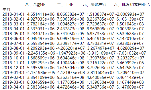
from statsmodels.tsa.seasonal import seasonal_decompose #周期性分解 def get_resid(ss): decomposition = seasonal_decompose(ss, period=12, two_sided=False) residual = decomposition.resid return residual #提取残差 resid={} for i in range(data_hy.shape[1]): resid[data_hy.columns[i]]=get_resid(data_hy.iloc[:,i]).values[12:].tolist() resid_hy=pd.DataFrame.from_dict(resid) resid_hy['年月']=data_wb.iloc[12:,].index resid_hy =resid_hy.set_index('年月') print(resid_hy )

部分结果预览。已过滤掉Nan值

3、目标变量残差与外部宏观经济或气象数据相关性分析

依次计算各目标变量与全部影响因素变量的皮尔逊相关系数，生成相关系数矩阵

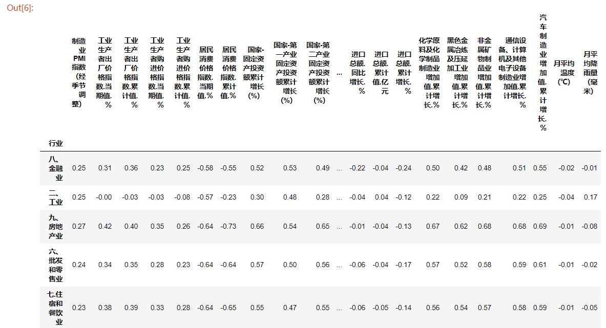
#相关系数矩阵 ss={} for i in range(data_wb.iloc[12:,].shape[1]): v=[] for j in range(resid_hy.shape[1]): v.append(round(resid_hy.iloc[:,j].corr(data_wb.iloc[12:,].iloc[:,i]),2)) ss[data_wb.iloc[12:,].columns[i]] = v df_hy=pd.DataFrame.from_dict(ss) df_hy['行业']=resid_hy.columns df_hy =df_hy.set_index('行业') print(df_hy)

部分结果预览。其中横向表头为影响因素变量名称，纵向表头为目标变量名称，纵横交叉单元格中数值即为该目标变量与该影响因素相关系数值

为直观观察各目标变量与影响因素之间的相关程度，绘制相关系数矩阵热力图

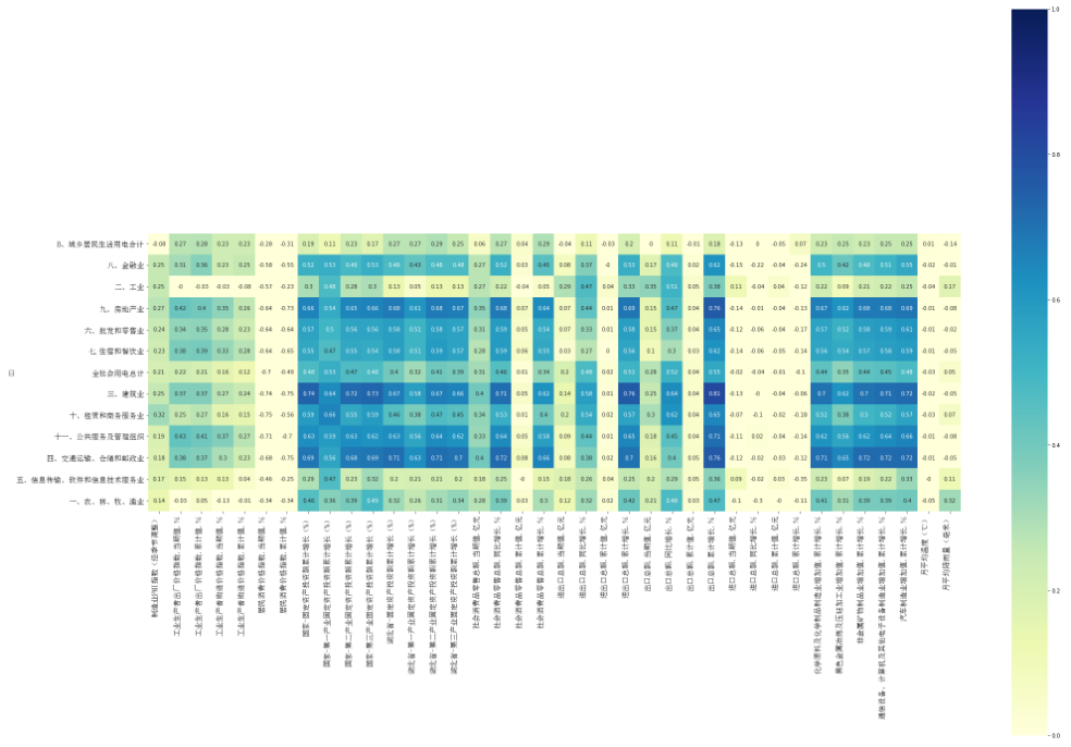
import seaborn as sns import matplotlib.pyplot as plt from matplotlib.font_manager import FontProperties #中文字符显示 font = FontProperties(fname=r"c:\windows\fonts\simsun.ttc", size=14) #相关系数矩阵热力图 fig, ax = plt.subplots(figsize = (30,20)) sns.heatmap(df_hy, annot=True, vmax=1,vmin = 0, xticklabels= True, yticklabels= True, square=True, cmap="YlGnBu") ax.set_yticklabels(df_hy.index, fontsize = 18, rotation = 360, horizontalalignment='right',fontproperties=font) ax.set_xticklabels(df_hy.columns, fontsize = 18, horizontalalignment='right',fontproperties=font) plt.tight_layout() plt.show()

如图所示，颜色由深蓝到亮黄，相关系数从高度正相关渐变为不相关、然后再渐变为高度负相关。本例中并没有观察到显著的相关性。

二、时序数据建模预测

1、目标变量时序数据周期分解

1.1、样本数据获取

本例目标变量为某地区多个行业电量数据，为降低复杂度选取其中一个行业进行说明，读取目标变量时序数据后将“年月”字段设置为索引。

import pandas as pd # 加载数据 data_dl = pd.read_excel("C:/Users/admin/Desktop/=data.xlsx",sheet_name='目标变量') data_dl['年月']=data_dl['年月'].astype(object) data_dl['年月'] = pd.to_datetime(data_dl['年月'],format='%Y%m') data_dl =data_dl.set_index('年月') ts_data=data_dl['目标变量1']

1.2、目标变量时序数据周期分解与残差界限

将目标变量时序数据进行周期性分解，分别获取trend趋势部分、seasonal周期部分、residual残差部分。计算得到low_error残差下界与high_error残差上界。

#周期性分解 from statsmodels.tsa.seasonal import seasonal_decompose decomposition = seasonal_decompose(ts_data, period=12, two_sided=False) trend = decomposition.trend seasonal = decomposition.seasonal residual = decomposition.resid #随机部分-误差界限 rdes=residual.describe() delta = rdes['75%'] - rdes['25%'] low_error, high_error = (rdes['25%'] - 1 * delta, rdes['75%'] + 1 * delta)

1.3、原始序列与周期性分解序列对比分布图

为直观观察目标变量原始序列与分解后的trend、seasonal、residual序列规律特征，绘制对比分布图。

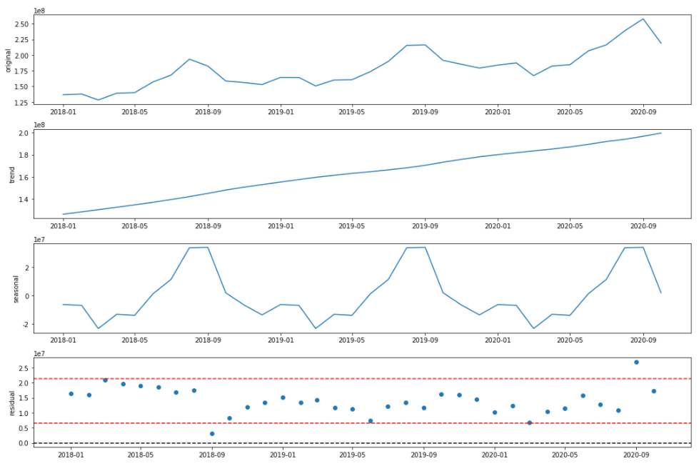
import matplotlib.pyplot as plt #周期分解绘图 plt.figure(figsize=(15,10)) plt.subplot(411) plt.plot(ts_data.index[12:],ts_data[12:]) plt.ylabel('original') plt.subplot(412) plt.plot(ts_data.index[12:],trend[12:]) plt.ylabel('trend') plt.subplot(413) plt.plot(ts_data.index[12:],seasonal[12:]) plt.ylabel('seasonal') plt.subplot(414) plt.scatter(ts_data.index[12:],residual[12:]) plt.ylabel('residual') plt.axhline(0,color='black',ls='--') plt.axhline(high_error,color='red',ls='--') plt.axhline(low_error,color='red',ls='--') plt.tight_layout() plt.show()

如图所示，依次展示目标变量original与trend、seasonal、residual序列分布图，已过滤掉Nan值。可以看到原始序列具有明显的周期变化规律，趋势部分呈稳步上升规律，周期部分各月数值比较稳定，残差部分基本均为正值、红线为残差界限。

2、trend趋势序列ARIMA建模预测

2.1、trend序列平稳性检验

使用单位根方法检验trend序列的平稳性，若为非平稳序列，则对序列进行d阶差分处理后再次检验，本例trend序列经1阶差分后达到平稳，即d=1。

import numpy as np # 进行d阶差分运算 test_len=3 d = 1 z = [] for t in range(d,trend[12:-test_len].shape[0]): tmp = 0 for i in range(0,d+1): tmp = tmp + (-1)i*(np.math.factorial(d)/(np.math.factorial(i)*np.math.factorial(d-i)))*trend[12:][t-i] z.append(tmp) # 使用单位根检验差分后序列的平稳性 import statsmodels.tsa.stattools as stat print(stat.adfuller(z, 1))

检验结果示例，由于检验结果的P值小于0.05，因此认为经d阶差分后的序列是平稳的。

2.2、trend平稳序列白噪声检验

使用Ljung-Box方法检验trend平稳序列是否为白噪声，若为白噪声则认为该序列已无任何有用信息残存、对其建模没有意义。

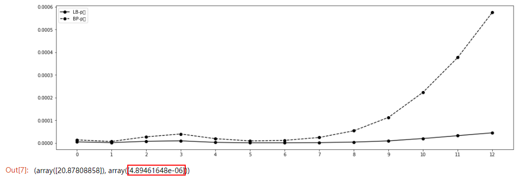
from statsmodels.stats.diagnostic import acorr_ljungbox as lb_test import warnings #Ljung_Box白噪声检验 warnings.filterwarnings("ignore") plt.figure(figsize=(15,5)) plt.plot(lb_test(z,boxpierce=True)[1],'o-',c='black',label="LB-p值") plt.plot(lb_test(z,boxpierce=True)[3],'o--',c='black',label="BP-p值") label=np.arange(0, len(lb_test(z,boxpierce=True)[1]), step=1) plt.xticks(label) plt.legend() plt.tight_layout() plt.show() print(lb_test(z, lags=1))

检验结果示例，由于检验结果的P值小于0.05，因此得出：经过d阶差分后的trend序列是一个平稳非白噪声的序列，适合建模预测。

2.3、trend平稳非白噪序列ARIMA模型定阶

绘制trend平稳非白噪序列的pacf图与acf图，根据pacf与acf的性质估计序列的自相关阶数p值与移动平均阶数q值。

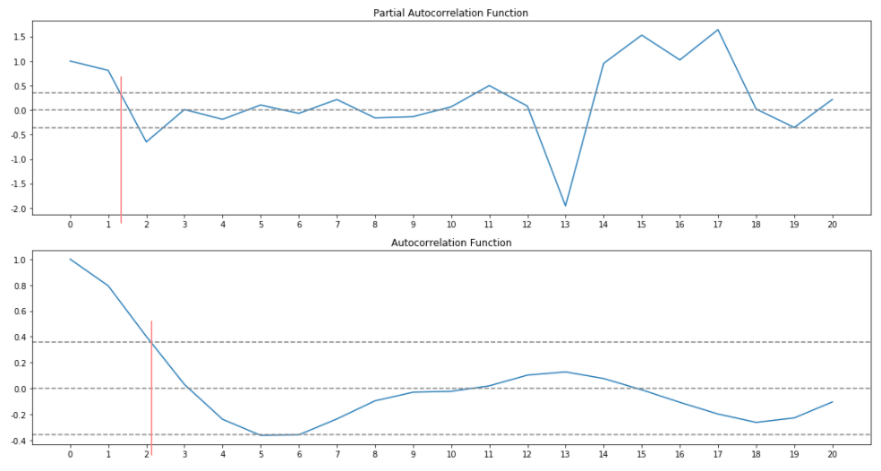
from statsmodels.tsa.stattools import acf, pacf plt.rcParams['axes.unicode_minus']=False fig, axes = plt.subplots(nrows=2, ncols=1,figsize=(15,8)) ax0, ax1 = axes.flatten() #模型定阶：p值 lag_pacf = pacf(z, nlags=20, method='ols') ax0.plot(lag_pacf) label=np.arange(0, 21, step=1) ax0.set_xticks(label) ax0.axhline(y=0, linestyle='--', color='gray') ax0.axhline(y=-1.96 / np.sqrt(len(z)), linestyle='--', color='gray')# lowwer置信区间 ax0.axhline(y=1.96 / np.sqrt(len(z)), linestyle='--', color='gray')# upper置信区间 ax0.set_title('Partial Autocorrelation Function') #模型定阶：q值 lag_acf = acf(z, nlags=20) ax1.plot(lag_acf) label=np.arange(0, 21, step=1) ax1.set_xticks(label) ax1.axhline(y=0, linestyle='--', color='gray') ax1.axhline(y=-1.96 / np.sqrt(len(z)), linestyle='--', color='gray') # lowwer置信区间 ax1.axhline(y=1.96 / np.sqrt(len(z)), linestyle='--', color='gray') # upper置信区间 ax1.set_title('Autocorrelation Function') plt.tight_layout() plt.show()

如图所示，pacf图中曲线第一次穿过上置信界限对应的横轴值约为1，即p=1；acf图中曲线第一次穿过上置信界限对应的横轴值约为2，即q=2。

2.4、trend平稳非白噪序列ARIMA模型预测

前文得到d=1，p=1，q=2，因此ARIMA(p,d,q)=ARIMA(1,1,2)，即ARIMA模型参数order=(1,1,2)。

构建ARIMA模型，在训练集上完成模型训练，在测试集上验证模型效果，计算预测准确率。

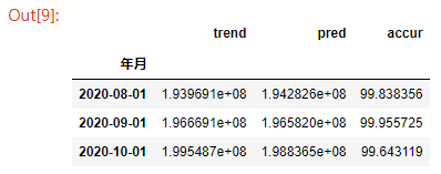
from statsmodels.tsa.arima_model import ARIMA #划分训练集与测试集，训练模型，评估模型效果 order=(1,1,2) trend_train = trend[12:-test_len] trend_test = trend[-test_len:] trend_model = ARIMA(trend_train, order=order).fit(disp=-1, method='css') trend_pred= trend_model.forecast(test_len)[0] ss_trend=pd.Series(trend_pred,index=trend_test.index,name='pred') result_trend = pd.concat([trend_test, ss_trend], axis=1) result_trend['accur']=100-abs((result_trend['pred']-result_trend[trend_test.name])*100/result_trend[trend_test.name]) print(result_trend)

如下表所示，ARIMA模型在trend序列测试集上的预测准确率。

3、residual残差序列Lasso回归建模预测

3.1、样本宽表数据获取

将residual残差序列过滤Nan值后作为目标变量y；本例影响因素宽表为某地区宏观经济与气象数据，根据年月与目标变量对齐，读取影响因素时序数据后将“年月”字段设置为索引，作为自变量x；划分训练集与测试集。

#加载影响因素数据 data_wb = pd.read_excel("C:/Users/admin/Desktop/data.xlsx",sheet_name='外部影响因素') data_wb['年月']=data_wb['年月'].astype(object) data_wb['年月'] = pd.to_datetime(data_wb['年月'],format='%Y%m') data_wb =data_wb.set_index('年月') #自变量、因变量 x = data_wb.iloc[12:,] y = residual.iloc[12:,] #划分训练集、测试集 x_train = x[:-test_len].copy() x_test=x[-test_len:].copy() y_train = y[:-test_len].copy() y_test=y[-test_len:].copy()

3.2、基于外部宏观经济与气象数据的residual残差回归模型构建

通过交叉验证获取Lasso模型参数alpha最优值，在训练集上构建模型、完成模型训练。输出alpha与回归系数。

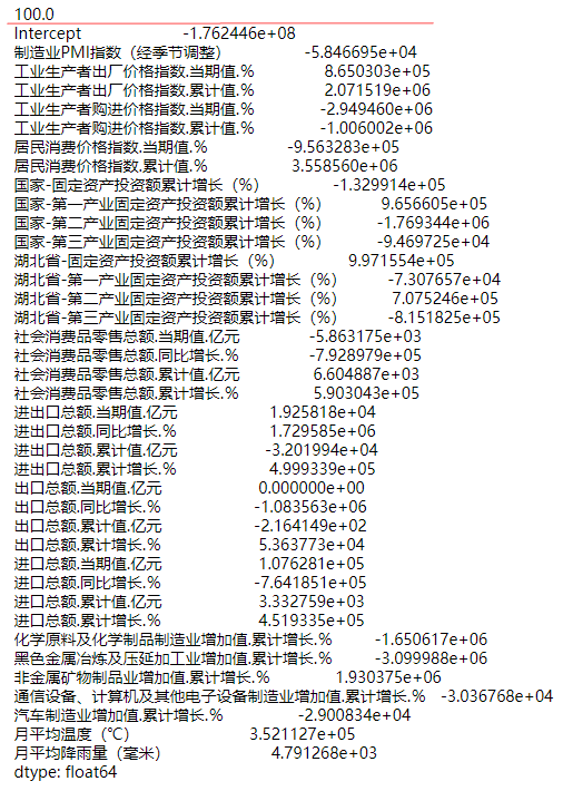
from sklearn.linear_model import LassoCV,Lasso # 获取最佳alpha参数值 Lambdas = np.logspace(-5, 2, 200) lasso_cv = LassoCV(alphas = Lambdas, normalize=True, cv = 10, max_iter=10000) lasso_cv.fit(x_train, y_train) lasso_best_alpha = lasso_cv.alpha_ # 基于最佳alpha值建模 lasso = Lasso(alpha = lasso_best_alpha, normalize=True, max_iter=10000) lasso.fit(x_train, y_train) #系数、截距 coeffiecients=pd.Series(index = ['Intercept'] + x_train.columns.tolist(),data = [lasso.intercept_] + lasso.coef_.tolist()) print(lasso_cv.alpha_) print(coeffiecients) 

如下所示，Lasso模型alpha值为100；回归系数包含截距值Intercept与各影响因素权重值。

3.3、residual残差序列Lasso回归模型评估

在测试集上验证模型效果，计算预测准确率。

#评估模型 resid_pred = lasso.predict(x_test) ss_resid=pd.Series(resid_pred,index=y_test.index,name='pred') result_resid = pd.concat([y_test, ss_resid], axis=1) result_resid['accur']=100-abs((result_resid['pred']-result_resid[y_test.name])*100/result_resid[y_test.name]) print(result_resid)

如下表所示：Lasso模型在residual序列测试集上的预测准确率（影响因素找的比较泛，针对性不强，因此模型表现很一般）。

4、叠加生成目标变量原始时序数据预测结果

前文对具有明显季节规律的目标变量原始时序数据拆分成趋势部分、周期部分、残差部分。趋势部分取ARIMA预测值；周期部分各月同期值较稳定，预测月份直接取该月份历年平均值；残差部分分别取0值、残差下界值、残差上界值、Lasso回归预测值。

叠加趋势部分与周期部分后，依次与残差部分不同方案值叠加生成目标变量整体预测值的不同方案结果，即：

趋势部分+周期部分+0=目标变量整体预测值中方案final_pred；

趋势部分+周期部分+残差下界值=目标变量整体预测值低方案low_conf；

趋势部分+周期部分+残差上界值=目标变量整体预测值高方案high_conf；

趋势部分+周期部分+Lasso回归预测值=目标变量整体预测值多模型融合方案compre_conf；

在测试集上验证模型效果，计算各方案预测准确率。实际应用中，将根据行业当前发展态势或结合其他因素，经判断后选取最合理的方案结果作为最终预测结果。

#为趋势预测值叠加周期部分及随机部分 predict_values = [] low_conf_values = [] high_conf_values = [] compre_values = [] for i, t in enumerate(y_test.index): #趋势部分 trend_part = ss_trend[i] #周期部分，取历史所有该月份的平均值 season_part = seasonal[seasonal.index.month == t.month].mean() #残差部分 residual_part = ss_resid[i] #趋势部分叠加周期部分 predict = trend_part + season_part #叠加误差下限 low_bound = predict + low_error #叠加误差上限 high_bound = predict + high_error #叠加残差回归结果 compre= predict +residual_part #追加n期结果 predict_values.append(predict) low_conf_values.append(low_bound) high_conf_values.append(high_bound) compre_values.append(compre) #结果输出格式转换 final_pred = pd.Series(predict_values, index=y_test.index, name='predict') low_conf = pd.Series(low_conf_values, index=y_test.index, name='low_conf') high_conf = pd.Series(high_conf_values, index=y_test.index, name='high_conf') compre_conf = pd.Series(compre_values, index=y_test.index, name='compre_conf') #准确率 predict_describe=pd.concat([ts_data,final_pred, low_conf, high_conf,compre_conf], axis=1) predict_describe['dev']=100-abs((predict_describe['predict']-predict_describe[ts_data.name])*100/predict_describe[ts_data.name]) predict_describe['dev_h']=100-abs((predict_describe['high_conf']-predict_describe[ts_data.name])*100/predict_describe[ts_data.name]) predict_describe['dev_l']=100-abs((predict_describe['low_conf']-predict_describe[ts_data.name])*100/predict_describe[ts_data.name]) predict_describe['dev_c']=100-abs((predict_describe['compre_conf']-predict_describe[ts_data.name])*100/predict_describe[ts_data.name]) print(predict_describe.iloc[-test_len:,])

如下表所示：本例重点考虑季节影响特征，在9月、10月会选取高方案结果（8月随便选吧）。

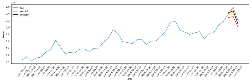
为直观查看、对比各种方案预测结果与实际值的差距，绘制目标变量实际值曲线（蓝色）、预测结果中方案曲线（红色）、多模型融合预测结果曲线（黑色）、预测结果低方案与高方案填充图（透明橙色）。

#绘图观察结果，高方案、低方案、中方案、综合多模型结果 plt.figure(figsize=(15,5)) plt.plot(predict_describe.index,predict_describe[ts_data.name],label='real') plt.plot(predict_describe.index,predict_describe['predict'],label='predict',c='red', linewidth=2) plt.plot(predict_describe.index,predict_describe['compre_conf'],label='compre',c='k', linewidth=2) plt.fill_between(predict_describe.index, predict_describe['low_conf'], predict_describe['high_conf'],color='orange',alpha=.25) plt.xticks(predict_describe.index,rotation=50) plt.xlabel('date') plt.ylabel('target') plt.legend() plt.tight_layout() plt.show()

如图所示：