
大家好,又见面了,我是你们的朋友全栈君。

I’m trying to port some MatLab code over to Scipy, and I’ve tried two different functions from scipy.interpolate, interp1d and UnivariateSpline. The interp1d results match the interp1d MatLab function, but the UnivariateSpline numbers come out different – and in some cases very different.
f = interp1d(row1,row2,kind=’cubic’,bounds_error=False,fill_value=numpy.max(row2))
return f(interp)
f = UnivariateSpline(row1,row2,k=3,s=0)
return f(interp)
Could anyone offer any insight? My x vals aren’t equally spaced, although I’m not sure why that would matter.
解决方案
I just ran into the same issue.
Short answer
f = InterpolatedUnivariateSpline(row1, row2)
return f(interp)
Long answer
UnivariateSpline is a ‘one-dimensional smoothing spline fit to a given set of data points’ whereas InterpolatedUnivariateSpline is a ‘one-dimensional interpolating spline for a given set of data points’. The former smoothes the data whereas the latter is a more conventional interpolation method and reproduces the results expected from interp1d. The figure below illustrates the difference.
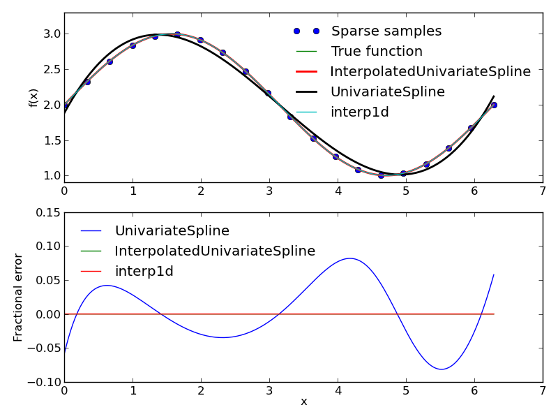
The code to reproduce the figure is shown below.
import scipy.interpolate as ip
#Define independent variable
sparse = linspace(0, 2 * pi, num = 20)
dense = linspace(0, 2 * pi, num = 200)
#Define function and calculate dependent variable
f = lambda x: sin(x) + 2
fsparse = f(sparse)
fdense = f(dense)
ax = subplot(2, 1, 1)
#Plot the sparse samples and the true function
plot(sparse, fsparse, label = ‘Sparse samples’, linestyle = ‘None’, marker = ‘o’)
plot(dense, fdense, label = ‘True function’)
#Plot the different interpolation results
interpolate = ip.InterpolatedUnivariateSpline(sparse, fsparse)
plot(dense, interpolate(dense), label = ‘InterpolatedUnivariateSpline’, linewidth = 2)
smoothing = ip.UnivariateSpline(sparse, fsparse)
plot(dense, smoothing(dense), label = ‘UnivariateSpline’, color = ‘k’, linewidth = 2)
ip1d = ip.interp1d(sparse, fsparse, kind = ‘cubic’)
plot(dense, ip1d(dense), label = ‘interp1d’)
ylim(.9, 3.3)
legend(loc = ‘upper right’, frameon = False)
ylabel(‘f(x)’)
#Plot the fractional error
subplot(2, 1, 2, sharex = ax)
plot(dense, smoothing(dense) / fdense – 1, label = ‘UnivariateSpline’)
plot(dense, interpolate(dense) / fdense – 1, label = ‘InterpolatedUnivariateSpline’)
plot(dense, ip1d(dense) / fdense – 1, label = ‘interp1d’)
ylabel(‘Fractional error’)
xlabel(‘x’)
ylim(-.1,.15)
legend(loc = ‘upper left’, frameon = False)
tight_layout()
发布者:全栈程序员-站长,转载请注明出处:https://javaforall.net/131821.html原文链接:https://javaforall.net


