
大家好,又见面了,我是你们的朋友全栈君。
图像降噪算法——从BM3D到VBM4D
图像降噪算法——从BM3D到VBM4D
BM3D算法是目前非AI降噪算法中最经典的算法之一,在BM3D的框架上改进得到的算法不计其数,这篇论文主要将BM3D算法的算法框架,在此基础上在结论中补充了下VBM3D算法和VBM4D算法。
1. 基本原理
BM3D算法的算法流程图如下所示:
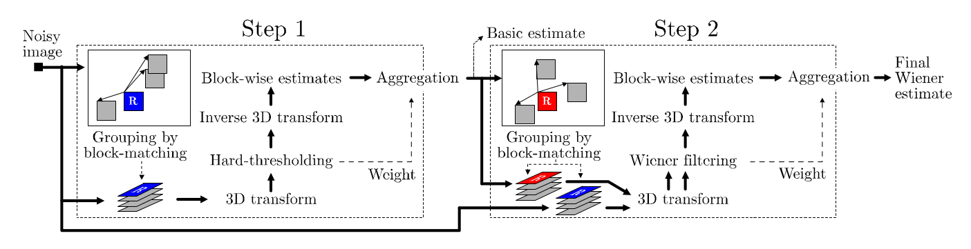

如图所示,算法一共分为两阶段,第一阶段主要实现了一个基于patch的硬阈值滤波,第二阶段主要实现了一个基于patch的维纳滤波,这里注意,BM3D的处理都是基于patch进行的,其中硬阈值滤波的过程只是一个预滤波的过程,而实际的降噪结果是来自于第二阶段的维纳滤波。下面我们对算法流程进行一个详细解释。
第一阶段:硬阈值滤波
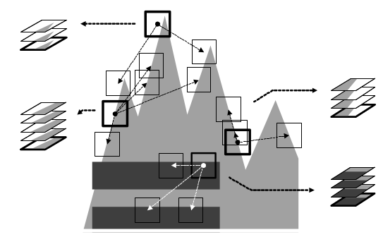
(1)在原始噪声图像上,在目标patch周围搜索相似的图像patch,这里的相似定义为两个图像patch像素简单L2距离,将相似的patch组合成一个个group,这里要注意,在组合group的同时,需要记录group中的各个patch在原始图像上的坐标,因为在第一阶段结束的Aggregation过程中需要将降噪后的图像patch重构为原始的图像,论文中的这个示意图就很好地说明了这个过程2
在论文中该过程抽象为如下两个公式: d noisy ( Z x R , Z x ) = ∥ Z x R − Z x ∥ 2 2 ( N 1 h t ) 2 d^{\text {noisy }}\left(Z_{x_{R}}, Z_{x}\right)=\frac{\left\|Z_{x_{R}}-Z_{x}\right\|_{2}^{2}}{\left(N_{1}^{\mathrm{ht}}\right)^{2}} dnoisy (ZxR,Zx)=(N1ht)2∥ZxR−Zx∥22 S x R h t = { x ∈ X : d ( Z x R , Z x ) ≤ τ match h t } S_{x_{R}}^{\mathrm{ht}}=\left\{x \in X: d\left(Z_{x_{R}}, Z_{x}\right) \leq \tau_{\text {match }}^{\mathrm{ht}}\right\} SxRht={
x∈X:d(ZxR,Zx)≤τmatch ht}
(2)接下来是在group上进行硬阈值滤波,硬阈值滤波相关的内容可以参考我之前的博客图像降噪算法——小波硬阈值滤波(上)和图像降噪算法——小波硬阈值滤波(下),大致原理是相同的。不同的是,因为这里的group是3D的元素结构,因此我们需要对group进行3D变换,3D变换是由一个2D的DCT变换或者Bior变换加上一个1D的Haar变换构成的。在3D变换的基础上进行硬阈值滤波,在完成硬阈值滤波后再进行3D反变换即可,该过程在论文中抽象为如下公式: Y ^ S x R h t = T 3 D h t − 1 ( Υ ( T 3 D h t ( Z S x R h t ) ) ) \widehat{\mathbf{Y}}_{S_{x_{R}}^{\mathrm{ht}}}=\mathcal{T}_{3 \mathrm{D}}^{\mathrm{ht}^{-1}}\left(\Upsilon\left(\mathcal{T}_{3 \mathrm{D}}^{\mathrm{ht}}\left(\mathbf{Z}_{S_{x_{R}}^{\mathrm{ht}}}\right)\right)\right) Y
SxRht=T3Dht−1(Υ(T3Dht(ZSxRht)))
(3)最后进行聚合(aggregation)操作,我们完成硬阈值滤波后得到仍然是一个个的group,聚合操作就是根据记录的各个patch中的坐标将group恢复成完整图像,在恢复过程中可能存在patch间overlap的情况,这时候会对patch的overlap部分进行加权平均,权重来自于硬阈值滤波过程中的系数
第二阶段:维纳滤波
(1)在第一阶段预降噪后的图像上,在目标patch周围搜索相似patch,然后构建group,公式如下: S x R wie = { x ∈ X : ∥ Y ^ x R basic − Y ^ x basic ∥ 2 2 ( N 1 wie ) 2 < τ match wie } S_{x_{R}}^{\text {wie }}=\left\{x \in X: \frac{\left\|\widehat{Y}_{x_{R}}^{\text {basic }}-\widehat{Y}_{x}^{\text {basic }}\right\|_{2}^{2}}{\left(N_{1}^{\text {wie }}\right)^{2}}<\tau_{\text {match }}^{\text {wie }}\right\} SxRwie =⎩⎪⎨⎪⎧x∈X:(N1wie )2∥∥∥Y
xRbasic −Y
xbasic ∥∥∥22<τmatch wie ⎭⎪⎬⎪⎫不同的,因为第二阶段用到的是维纳滤波,我们一共需要构建两组group,第一组group就是如上所述的在预降噪图像上搜索得到的,第二组group是按照同样的坐标,在原始噪声图像进行构建。
(2)接下来是进行维纳滤波,维纳滤波的相关内容可以参考图像降噪算法——维纳滤波,维纳滤波公式如下: W S x R wie = ∣ T 3 D wie ( Y ^ S x wie basic ) ∣ 2 ∣ T 3 D wie ( Y ^ S x wic basic ) ∣ 2 + σ 2 \mathbf{W}_{S_{x_{R}}^{\text {wie }}}= \frac{\left|\mathcal{T}_{3 \mathrm{D}}^{\text {wie }}\left(\widehat{\mathbf{Y}}_{S_{x}^{\text {wie }}}^{\text {basic }}\right)\right|^{2}}{\left|\mathcal{T}_{3 \mathrm{D}}^{\text {wie }}\left(\widehat{\mathbf{Y}}_{S_{x}^{\text {wic }}}^{\text {basic }}\right)\right|^{2}+\sigma^{2}} WSxRwie =∣∣∣T3Dwie (Y
Sxwic basic )∣∣∣2+σ2∣∣∣T3Dwie (Y
Sxwie basic )∣∣∣2 Y ^ S x R w i e = T 3 D w i e − 1 ( W S x R wie T 3 D wie ( Z S x R wie ) ) \widehat{\mathbf{Y}}_{S_{x_{R}}^{w i e}}=\mathcal{T}_{3 \mathrm{D}}^{\mathrm{wie}^{-1}}\left(\mathbf{W}_{S_{x_{R}}^{\text {wie }}} \mathcal{T}_{3 \mathrm{D}}^{\text {wie }}\left(\mathbf{Z}_{S_{x_{R}}^{\text {wie }}}\right)\right) Y
SxRwie=T3Dwie−1(WSxRwie T3Dwie (ZSxRwie ))可以看到,在维纳滤波我们是需要有输入图像的频谱作为降噪依据,在BM3D中就是采用第一阶段的预降噪图像作为输入图像
(3)最后同样是进行聚合(aggregation)操作,在overlap区域同样是进行加权平均,权重来自于维纳滤波系数,如下: w x R wie = σ − 2 ∥ W S x R wic ∥ 2 − 2 w_{x_{R}}^{\text {wie }}=\sigma^{-2}\left\|\mathbf{W}_{S_{x_{R}}^{\text {wic }}}\right\|_{2}^{-2} wxRwie =σ−2∥∥∥WSxRwic ∥∥∥2−2 y ^ basic ( x ) = ∑ x R ∈ X ∑ x m ∈ S x R h t w x R h t Y ^ x m h t , x R ( x ) ∑ x R ∈ X ∑ x m ∈ S x R h t w x R h t χ x m ( x ) , ∀ x ∈ X , \widehat{y}^{\text {basic }}(x)=\frac{\sum_{x_{R} \in X} \sum_{x_{m} \in S_{x_{R}}^{\mathrm{ht}}} w_{x_{R}}^{\mathrm{ht}} \widehat{Y}_{x_{m}}^{\mathrm{ht}, x_{R}}(x)}{\sum_{x_{R} \in X} \sum_{x_{m} \in S_{x_{R}}^{\mathrm{ht}}} w_{x_{R}}^{\mathrm{ht}} \chi_{x_{m}}(x)}, \forall x \in X, y
basic (x)=∑xR∈X∑xm∈SxRhtwxRhtχxm(x)∑xR∈X∑xm∈SxRhtwxRhtY
xmht,xR(x),∀x∈X,
以上就是BM3D算法的全部流程,可以看出来,BM3D算法实际上就是维纳滤波,但是其结合了NLM的思想,通过寻找相似patch加强了降噪的效果。
2. python代码实现
开源的BM3D算法C++代码也有,但是写得通常都比较复杂,这里我参考BM3D :稀疏三维变换域协同过滤的图像去噪||原理&算法实现提供一份python版本的实现,看完代码基本上就能屡清楚BM3D的实现过程了
# -*- coding: utf-8 -*-
""" *BM3D算法简单实现,主要程序部分 """
import cv2
import numpy
import math
import numpy.matlib

cv2.setUseOptimized(True)

# Parameters initialization
sigma = 25
Threshold_Hard3D = 2.7 * sigma  # Threshold for Hard Thresholding

Step1_Blk_Size = 4  # block_Size即块的大小
Step1_Blk_Step = 1  # Rather than sliding by one pixel to every next reference block, use a step of Nstep pixels in both horizontal and vertical directions.
Step1_Search_Step = 1  # 块的搜索step
First_Match_threshold = 125 * Step1_Blk_Size ** 2  # 用于计算block之间相似度的阈值
Step1_max_matched_cnt = 16  # 组最大匹配的块数
Step1_Search_Window = 15  # Search for candidate matching blocks in a local neighborhood of restricted size NS*NS centered

Step2_Blk_Size = 4
Step2_Blk_Step = 1
Step2_Search_Step = 1
Second_Match_threshold = 220. / 16 * Step2_Blk_Size ** 2  # 用于计算block之间相似度的阈值
Step2_max_matched_cnt = 32
Step2_Search_Window = 25

Beta_Kaiser = 1.5


def init(img, _blk_size, _Beta_Kaiser):
    """该函数用于初始化,返回用于记录过滤后图像以及权重的数组,还有构造凯撒窗"""
    m_shape = img.shape
    m_img = numpy.matrix(numpy.zeros(m_shape, dtype=float))
    m_wight = numpy.matrix(numpy.zeros(m_shape, dtype=float))

    # 窗函数(window function)是一种除在给定区间之外取值均为0的实函数
    K = numpy.matrix(numpy.kaiser(_blk_size, _Beta_Kaiser))
    m_Kaiser = numpy.array(K.T * K)  # 构造一个凯撒窗
    # 窗函数:https://zh.wikipedia.org/wiki/窗函数#Kaiser窗

    # print m_Kaiser, type(m_Kaiser), m_Kaiser.shape
    # cv2.imshow("Kaisser", m_Kaiser)
    # cv2.waitKey(0)
    # cv2.imwrite("Kaisser.jpg", m_Kaiser.astype(numpy.uint8))
    return m_img, m_wight, m_Kaiser


def Locate_blk(i, j, blk_step, block_Size, width, height):
    '''该函数用于保证当前的blk不超出图像范围'''
    if i * blk_step + block_Size < width:
        point_x = i * blk_step
    else:
        point_x = width - block_Size

    if j * blk_step + block_Size < height:
        point_y = j * blk_step
    else:
        point_y = height - block_Size

    m_blockPoint = numpy.array((point_x, point_y), dtype=int)  # 当前参考图像的顶点

    return m_blockPoint


def Define_SearchWindow(_noisyImg, _BlockPoint, _WindowSize, Blk_Size):
    """ 该函数利用block的左上顶点的位置返回一个二元组(x,y) 用以界定_Search_Window左上角顶点坐标 """
    point_x = _BlockPoint[0]  # 当前坐标
    point_y = _BlockPoint[1]  # 当前坐标

    # 获得SearchWindow四个顶点的坐标
    LX = point_x + Blk_Size / 2 - _WindowSize / 2  # 左上x
    LY = point_y + Blk_Size / 2 - _WindowSize / 2  # 左上y
    RX = LX + _WindowSize  # 右下x
    RY = LY + _WindowSize  # 右下y

    # 判断一下是否越界
    if LX < 0:
        LX = 0
    elif RX > _noisyImg.shape[0]:
        LX = _noisyImg.shape[0] - _WindowSize
    if LY < 0:
        LY = 0
    elif RY > _noisyImg.shape[0]:
        LY = _noisyImg.shape[0] - _WindowSize

    return numpy.array((LX, LY), dtype=int)


def Step1_fast_match(_noisyImg, _BlockPoint):
    """快速匹配"""
    ''' *返回邻域内寻找和当前_block相似度最高的几个block,返回的数组中包含本身 *_noisyImg:噪声图像 *_BlockPoint:当前block的坐标及大小 '''
    (present_x, present_y) = _BlockPoint  # 当前坐标
    Blk_Size = Step1_Blk_Size
    Search_Step = Step1_Search_Step
    Threshold = First_Match_threshold
    max_matched = Step1_max_matched_cnt
    Window_size = Step1_Search_Window

    blk_positions = numpy.zeros((max_matched, 2), dtype=int)  # 用于记录相似blk的位置
    Final_similar_blocks = numpy.zeros((max_matched, Blk_Size, Blk_Size), dtype=float)  # 用于保存最后结果

    img = _noisyImg[present_x: present_x + Blk_Size, present_y: present_y + Blk_Size]
    dct_img = cv2.dct(img.astype(numpy.float64))  # 对目标作block作二维余弦变换

    Final_similar_blocks[0, :, :] = dct_img  # 保存变换后的目标块
    blk_positions[0, :] = _BlockPoint

    Window_location = Define_SearchWindow(_noisyImg, _BlockPoint, Window_size, Blk_Size)
    blk_num = (Window_size - Blk_Size) / Search_Step  # 确定最多可以找到多少相似blk
    blk_num = int(blk_num)
    (present_x, present_y) = Window_location

    similar_blocks = numpy.zeros((blk_num ** 2, Blk_Size, Blk_Size), dtype=float)
    m_Blkpositions = numpy.zeros((blk_num ** 2, 2), dtype=int)
    Distances = numpy.zeros(blk_num ** 2, dtype=float)  # 记录各个blk与它的相似度

    # 开始在_Search_Window中搜索,初始版本先采用遍历搜索策略,这里返回最相似的几块
    matched_cnt = 0
    for i in range(blk_num):
        for j in range(blk_num):
            tem_img = _noisyImg[present_x: present_x + Blk_Size, present_y: present_y + Blk_Size]
            dct_Tem_img = cv2.dct(tem_img.astype(numpy.float64))
            # 先对块进行dct变换再求l2-norm,寻找相似块,降低噪点的干扰
            m_Distance = numpy.linalg.norm((dct_img - dct_Tem_img)) ** 2 / (Blk_Size ** 2)

            # 下面记录数据自动不考虑自身(因为已经记录)
            if m_Distance < Threshold and m_Distance > 0:  # 说明找到了一块符合要求的
                similar_blocks[matched_cnt, :, :] = dct_Tem_img
                m_Blkpositions[matched_cnt, :] = (present_x, present_y)
                Distances[matched_cnt] = m_Distance
                matched_cnt += 1
            present_y += Search_Step
        present_x += Search_Step
        present_y = Window_location[1]  # 搜索窗的行
    # 取前matched_cnt个块
    Distances = Distances[:matched_cnt]
    # 对distance进行排序,找到对应顺序的序号
    # numpy.argsort() 的用法:
    # https://docs.scipy.org/doc/numpy/reference/generated/numpy.argsort.html
    Sort = Distances.argsort()

    # 统计一下找到了多少相似的blk
    if matched_cnt < max_matched:
        Count = matched_cnt + 1
    else:
        Count = max_matched
    # 将前matched_cnt个块放入Final_similar_blocks,左上坐标信息保存在lk_positions
    if Count > 0:
        for i in range(1, Count):
            Final_similar_blocks[i, :, :] = similar_blocks[Sort[i - 1], :, :]
            blk_positions[i, :] = m_Blkpositions[Sort[i - 1], :]
    return Final_similar_blocks, blk_positions, Count


def Step1_3DFiltering(_similar_blocks):
    ''' *3D变换及滤波处理 *_similar_blocks:相似的一组block,这里已经是频域的表示 *要将_similar_blocks第三维依次取出,然在频域用阈值滤波之后,再作反变换 '''

    statis_nonzero = 0  # 非零元素个数
    m_Shape = _similar_blocks.shape

    # 下面这一段代码很耗时
    for i in range(m_Shape[1]):
        for j in range(m_Shape[2]):
            # print _similar_blocks[:, i, j], type(_similar_blocks[:, i, j])
            tem_Vct_Trans = cv2.dct(_similar_blocks[:, i, j])
            # 硬阈值变换,去掉较小的频率成分
            tem_Vct_Trans[numpy.abs(tem_Vct_Trans[:]) < Threshold_Hard3D] = 0.
            statis_nonzero += tem_Vct_Trans.nonzero()[0].size
            _similar_blocks[:, i, j] = cv2.idct(tem_Vct_Trans)[0]
    return _similar_blocks, statis_nonzero


def Aggregation_hardthreshold(_similar_blocks, blk_positions, m_basic_img, m_wight_img, _nonzero_num, Count, Kaiser):
    ''' *对3D变换及滤波后输出的stack进行加权累加,得到初步滤波的图片 *_similar_blocks:相似的一组block,这里是频域的表示 *对这些块,用非零项的权重乘以凯撒窗之后再分别放回原位 '''
    _shape = _similar_blocks.shape
    if _nonzero_num < 1:
        _nonzero_num = 1
    block_wight = (1. / (sigma ** 2 * _nonzero_num)) * Kaiser
    for i in range(Count):
        point = blk_positions[i, :]
        tem_img = block_wight * cv2.idct(_similar_blocks[i, :, :])
        m_basic_img[point[0]:point[0] + _shape[1], point[1]:point[1] + _shape[2]] += tem_img
        m_wight_img[point[0]:point[0] + _shape[1], point[1]:point[1] + _shape[2]] += block_wight


def BM3D_1st_step(_noisyImg):
    """第一步,基本去噪"""
    # 初始化一些参数:
    (width, height) = _noisyImg.shape  # width = row, height = col
    block_Size = Step1_Blk_Size  # 块大小
    blk_step = Step1_Blk_Step  # N块步长滑动
    # 根据步长确定搜索的次数
    Width_num = (width - block_Size) / blk_step
    Height_num = (height - block_Size) / blk_step

    # 初始化几个数组
    # 空图像、空权重表、凯撒窗
    Basic_img, m_Wight, m_Kaiser = init(_noisyImg, Step1_Blk_Size, Beta_Kaiser)

    # 开始逐block的处理,+2是为了避免边缘上不够
    for i in range(int(Width_num + 2)):
        for j in range(int(Height_num + 2)):
            # m_blockPoint当前参考图像的左上角顶点
            m_blockPoint = Locate_blk(i, j, blk_step, block_Size, width, height)  # 该函数用于保证当前的blk不超出图像范围
            Similar_Blks, Positions, Count = Step1_fast_match(_noisyImg, m_blockPoint)  # 相似块集合、相似块位置、相似块数量
            Similar_Blks, statis_nonzero = Step1_3DFiltering(Similar_Blks)  # 协同过滤后的相似块集合、非零项数量
            Aggregation_hardthreshold(Similar_Blks, Positions, Basic_img, m_Wight, statis_nonzero, Count, m_Kaiser)
    Basic_img[:, :] /= m_Wight[:, :]
    basic = numpy.matrix(Basic_img, dtype=int)
    basic.astype(numpy.uint8)

    return basic


def Step2_fast_match(_Basic_img, _noisyImg, _BlockPoint):
    ''' *快速匹配算法,返回邻域内寻找和当前_block相似度最高的几个block,要同时返回basicImg和IMG *_Basic_img: 基础去噪之后的图像 *_noisyImg:噪声图像 *_BlockPoint:当前block的坐标及大小 '''
    (present_x, present_y) = _BlockPoint  # 当前坐标
    Blk_Size = Step2_Blk_Size
    Threshold = Second_Match_threshold
    Search_Step = Step2_Search_Step
    max_matched = Step2_max_matched_cnt
    Window_size = Step2_Search_Window

    blk_positions = numpy.zeros((max_matched, 2), dtype=int)  # 用于记录相似blk的位置
    Final_similar_blocks = numpy.zeros((max_matched, Blk_Size, Blk_Size), dtype=float)
    Final_noisy_blocks = numpy.zeros((max_matched, Blk_Size, Blk_Size), dtype=float)

    img = _Basic_img[present_x: present_x + Blk_Size, present_y: present_y + Blk_Size]
    dct_img = cv2.dct(img.astype(numpy.float32))  # 对目标作block作二维余弦变换
    Final_similar_blocks[0, :, :] = dct_img

    n_img = _noisyImg[present_x: present_x + Blk_Size, present_y: present_y + Blk_Size]
    dct_n_img = cv2.dct(n_img.astype(numpy.float32))  # 对目标作block作二维余弦变换
    Final_noisy_blocks[0, :, :] = dct_n_img

    blk_positions[0, :] = _BlockPoint

    Window_location = Define_SearchWindow(_noisyImg, _BlockPoint, Window_size, Blk_Size)
    blk_num = (Window_size - Blk_Size) / Search_Step  # 确定最多可以找到多少相似blk
    blk_num = int(blk_num)
    (present_x, present_y) = Window_location

    similar_blocks = numpy.zeros((blk_num ** 2, Blk_Size, Blk_Size), dtype=float)
    m_Blkpositions = numpy.zeros((blk_num ** 2, 2), dtype=int)
    Distances = numpy.zeros(blk_num ** 2, dtype=float)  # 记录各个blk与它的相似度

    # 开始在_Search_Window中搜索,初始版本先采用遍历搜索策略,这里返回最相似的几块
    matched_cnt = 0
    for i in range(blk_num):
        for j in range(blk_num):
            tem_img = _Basic_img[present_x: present_x + Blk_Size, present_y: present_y + Blk_Size]
            # dct_Tem_img = cv2.dct(tem_img.astype(numpy.float32))
            # m_Distance = numpy.linalg.norm((dct_img - dct_Tem_img)) ** 2 / (Blk_Size ** 2)

            m_Distance = numpy.linalg.norm((img - tem_img)) ** 2 / (Blk_Size ** 2)
            # 下面记录数据自动不考虑自身(因为已经记录)
            if m_Distance < Threshold and m_Distance > 0:
                dct_Tem_img = cv2.dct(tem_img.astype(numpy.float32))
                similar_blocks[matched_cnt, :, :] = dct_Tem_img
                m_Blkpositions[matched_cnt, :] = (present_x, present_y)
                Distances[matched_cnt] = m_Distance
                matched_cnt += 1
            present_y += Search_Step
        present_x += Search_Step
        present_y = Window_location[1]
    Distances = Distances[:matched_cnt]
    Sort = Distances.argsort()

    # 统计一下找到了多少相似的blk
    if matched_cnt < max_matched:
        Count = matched_cnt + 1
    else:
        Count = max_matched

    # nosiy图像的3D Stack,利用第一步的Basic估计结果来构造
    if Count > 0:
        for i in range(1, Count):
            Final_similar_blocks[i, :, :] = similar_blocks[Sort[i - 1], :, :]
            blk_positions[i, :] = m_Blkpositions[Sort[i - 1], :]

            (present_x, present_y) = m_Blkpositions[Sort[i - 1], :]
            n_img = _noisyImg[present_x: present_x + Blk_Size, present_y: present_y + Blk_Size]
            Final_noisy_blocks[i, :, :] = cv2.dct(n_img.astype(numpy.float64))

    return Final_similar_blocks, Final_noisy_blocks, blk_positions, Count


def Step2_3DFiltering(_Similar_Bscs, _Similar_Imgs):
    ''' *3D维纳变换的协同滤波 *_similar_blocks:相似的一组block,这里是频域的表示 *要将_similar_blocks第三维依次取出,然后作dct,在频域进行维纳滤波之后,再作反变换 *返回的Wiener_wight用于后面Aggregation '''
    m_Shape = _Similar_Bscs.shape
    Wiener_wight = numpy.zeros((m_Shape[1], m_Shape[2]), dtype=float)

    for i in range(m_Shape[1]):
        for j in range(m_Shape[2]):
            tem_vector = _Similar_Bscs[:, i, j]
            tem_Vct_Trans = numpy.matrix(cv2.dct(tem_vector))

            Norm_2 = numpy.float64(tem_Vct_Trans.T * tem_Vct_Trans)
            m_weight = Norm_2 / (Norm_2 + sigma ** 2)
            Wiener_wight[i, j] = m_weight

            #if m_weight != 0: Wiener_wight[i, j] = 1. / (m_weight ** 2 * sigma ** 2)
            # else:
            # Wiener_wight[i, j] = 10000

            # RES=IDCT(WEIGHT(DCT(NOISE_BLOCK)))
            tem_vector = _Similar_Imgs[:, i, j]
            tem_Vct_Trans = m_weight * cv2.dct(tem_vector)
            _Similar_Bscs[:, i, j] = cv2.idct(tem_Vct_Trans)[0]

    return _Similar_Bscs, Wiener_wight


def Aggregation_Wiener(_Similar_Blks, _Wiener_wight, blk_positions, m_basic_img, m_wight_img, Count, Kaiser):
    ''' *对3D变换及滤波后输出的stack进行加权累加,得到初步滤波的图片 *_similar_blocks:相似的一组block,这里是频域的表示 *对于最后的块,乘以凯撒窗之后再输出 '''
    _shape = _Similar_Blks.shape
    block_wight = _Wiener_wight * Kaiser

    for i in range(Count):
        point = blk_positions[i, :]
        tem_img = _Wiener_wight * cv2.idct(_Similar_Blks[i, :, :]) * Kaiser
        m_basic_img[point[0]:point[0] + _shape[1], point[1]:point[1] + _shape[2]] += tem_img
        m_wight_img[point[0]:point[0] + _shape[1], point[1]:point[1] + _shape[2]] += block_wight


def BM3D_2nd_step(_basicImg, _noisyImg):
    '''Step 2. 最终的估计: 利用基本的估计,进行改进了的分组以及协同维纳滤波'''
    # 初始化一些参数:
    (width, height) = _noisyImg.shape
    block_Size = Step2_Blk_Size
    blk_step = Step2_Blk_Step
    Width_num = (width - block_Size) / blk_step
    Height_num = (height - block_Size) / blk_step

    # 初始化几个数组
    m_img, m_Wight, m_Kaiser = init(_noisyImg, block_Size, Beta_Kaiser)

    for i in range(int(Width_num + 2)):
        for j in range(int(Height_num + 2)):
            m_blockPoint = Locate_blk(i, j, blk_step, block_Size, width, height)
            Similar_Blks, Similar_Imgs, Positions, Count = Step2_fast_match(_basicImg, _noisyImg, m_blockPoint)
            Similar_Blks, Wiener_wight = Step2_3DFiltering(Similar_Blks, Similar_Imgs)
            Aggregation_Wiener(Similar_Blks, Wiener_wight, Positions, m_img, m_Wight, Count, m_Kaiser)
    m_img[:, :] /= m_Wight[:, :]
    Final = numpy.matrix(m_img, dtype=int)
    Final.astype(numpy.uint8)

    return Final


def Gauss_noise(img, sigma=25):
    noise = numpy.matlib.randn(img.shape) * sigma
    res = img + noise
    return res


def PSNR(img1, img2):
    D = numpy.array(img1 - img2, dtype=numpy.int64)
    D[:, :] = D[:, :] ** 2
    RMSE = D.sum() / img1.size
    psnr = 10 * math.log10(float(255. ** 2) / RMSE)
    return psnr


if __name__ == '__main__':
    cv2.setUseOptimized(True)  # OpenCV 中的很多函数都被优化过(使用 SSE2,AVX 等)。也包含一些没有被优化的代码。使用函数 cv2.setUseOptimized() 来开启优化。
    img_name = "./len128*128.jpg"  # 图像的路径
    ori = cv2.imread(img_name, cv2.IMREAD_GRAYSCALE)  # 读入图像,cv2.IMREAD_GRAYSCALE:以灰度模式读入图像
    cv2.imwrite("ori.jpg", ori)
    img = Gauss_noise(ori)
    cv2.imwrite("noise.jpg", img)

    print 'The PSNR After add noise %f' % PSNR(ori, img)
    # 记录程序运行时间
    e1 = cv2.getTickCount()  # cv2.getTickCount 函数返回从参考点到这个函数被执行的时钟数
    # if(img is not None):
    # print("success")
    Basic_img = BM3D_1st_step(img)
    e2 = cv2.getTickCount()
    time = (e2 - e1) / cv2.getTickFrequency()  # 计算函数执行时间
    print ("The Processing time of the First step is %f s" % time)
    cv2.imwrite("Basic3.jpg", Basic_img)

    print ("The PSNR between the two img of the First step is %f" % PSNR(ori, Basic_img))

    # Basic_img = cv2.imread("Basic3.jpg", cv2.IMREAD_GRAYSCALE)

    Final_img = BM3D_2nd_step(Basic_img, img)
    e3 = cv2.getTickCount()
    time = (e3 - e2) / cv2.getTickFrequency()
    print ("The Processing time of the Second step is %f s" % time)
    cv2.imwrite("Final3.jpg", Final_img)

    print ("The PSNR between the two img of the Second step is %f" % PSNR(ori, Final_img))
    time = (e3 - e1) / cv2.getTickFrequency()
    print ("The total Processing time is %f s" % time)
3. 结论
从BM3D提出之后,学术界就在BM3D的基础上涌现了一批类似的方法,例如最近2019年和2020年的唯一的两篇最新的TIP上的传统算法NLH和ACVA都是在BM3D的基础上改进的,还有一条很有意思的pipeline,就是BM3D -> BM4D -> VBM3D -> VBM4D这几个算法,其中:
BM4D算法框架如下:
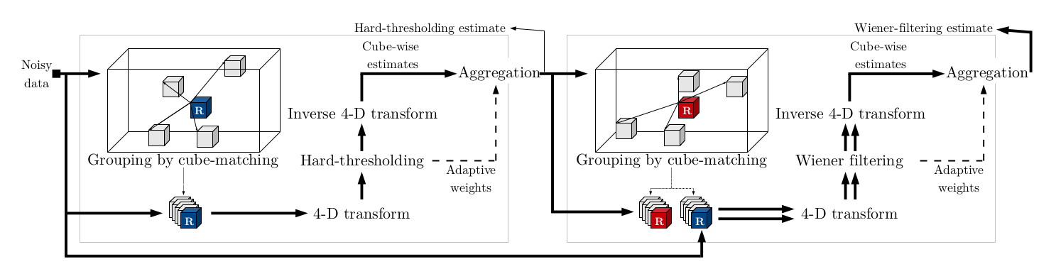
该算法仍然输入单帧降噪算法,不过对象不是二维图像,而是三维体素,在方法上应该没有什么太大的区别。
VBM3D算法框架如下:
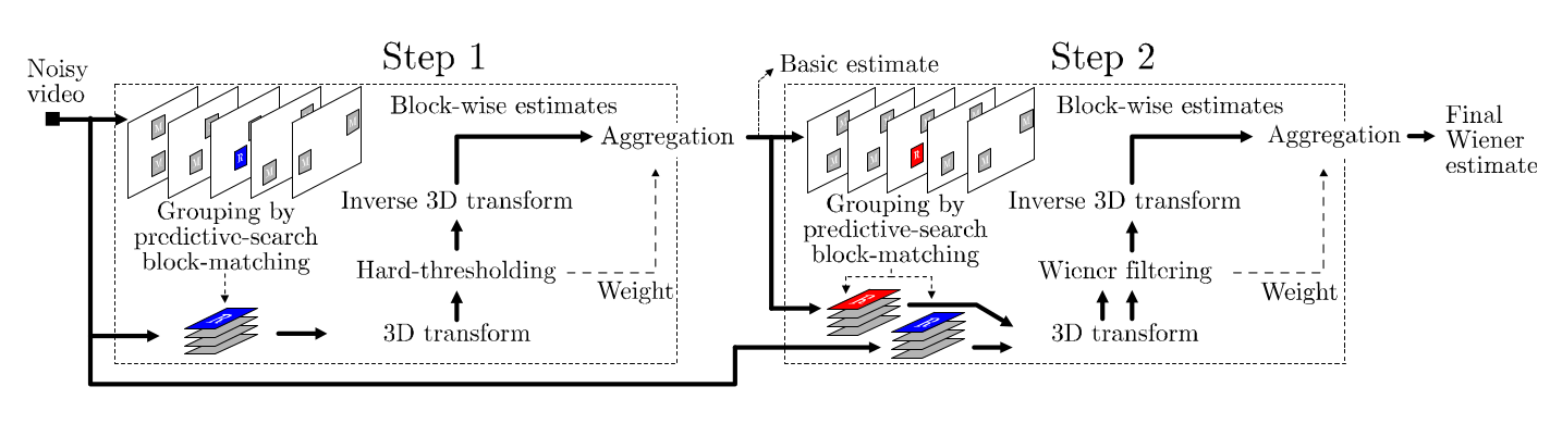
该算法属于时域去噪,在方法上没有太大的改变,如上图所示,只是在寻找相似patch时不是在单张图像上搜索,而是在相邻的若干张图像上进行搜索,仅仅是这样的变化,VBM3D也成了时域降噪领域里程碑式的算法,由此可见该算法的强大
VBM4D算法和VBM3D的算法主要的区别在于该算法对图像patch进行了对齐,此外在域变换的操作上也有相应的改进,具体的细节就不在此赘述了。
在工业界上,因为BM3D的计算量比较大,虽然效果好但实际用起来也确实很困难,在GPU上实现也很难达到实时,华为的麒麟芯片对该算法进行了硬化才达到实时降噪的效果
此外,这里我写一个各种算法的总结目录图像降噪算法——图像降噪算法总结,对图像降噪算法感兴趣的同学欢迎参考
发布者:全栈程序员-站长,转载请注明出处:https://javaforall.net/135159.html原文链接:https://javaforall.net


