
大家好,又见面了,我是你们的朋友全栈君。如果您正在找激活码,请点击查看最新教程,关注关注公众号 “全栈程序员社区” 获取激活教程,可能之前旧版本教程已经失效.最新Idea2022.1教程亲测有效,一键激活。
Jetbrains全系列IDE稳定放心使用

SiamFC
https://zhuanlan.zhihu.com/p/66757733?utm_source=wechat_session
特征提取网络
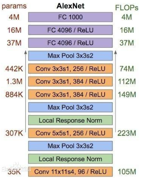
siamfc 特征提取网络是以 Alexnet 为基础的,通过 Alexnet 构建孪生网络
    def __init__(self, gpu_id, train=True):
        super(SiameseAlexNet, self).__init__()
        self.features = nn.Sequential(
            nn.Conv2d(3, 96, 11, 2),            #(1)Conv1  stride=2 第一个卷积层--输入通道,输出通道,卷积核的大小,(stride)步长
            nn.BatchNorm2d(96),     #输入通道
            nn.ReLU(inplace=True),  #
            nn.MaxPool2d(3, 2),                 #Pool1  stride=2 卷积核大小,stride步长
            nn.Conv2d(96, 256, 5, 1, groups=2), #(2)Conv2  stride=2    对于每一个组输入是48 第二个卷积层
            nn.BatchNorm2d(256),  #输入通道,
            nn.ReLU(inplace=True),
            nn.MaxPool2d(3, 2),                 #Pool2 stride=2
            nn.Conv2d(256, 384, 3, 1),          #(3)Conv3
            nn.BatchNorm2d(384),
            nn.ReLU(inplace=True),
            nn.Conv2d(384, 384, 3, 1, groups=2),#(4)Conv4 groups分成两个组,对于每一个组输入是192
            nn.BatchNorm2d(384),
            nn.ReLU(inplace=True),
            nn.Conv2d(384, 256, 3, 1, groups=2) #(5)Conv5
        )
        self.corr_bias = nn.Parameter(torch.zeros(1)) # Parameter
孪生网络讲解
这里的孪生网络和siamfc的区别??
- 传统孪生网络的输出输出相同,而siamfc输入输出不同
- 传统孪生网络的传递函数,两输入相同,则输出的向量距离越近,输出不同,输出的向量距离越远。根据这个思想,相同图像,标签为1,不同图像,标签为0,而siamfc标签如何构造?
SiamFC孪生网络细解
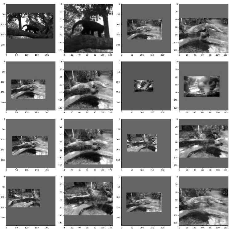
**首先看幅原论文图像,这里图像直接从其他博客,截图过来的,发现他提的问题挺有意思。前期,我读论文时,也别这幅图给严重误导,阅读代码,调试后,我可以得到这样一幅图
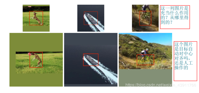
着幅黑白图,是跑出来的结果,图C是原图,而输入孪生网络的是图a,和图b,图a是你跟踪是第一帧选的框.意不意外,惊不惊喜原图没有通过网络,这也是此算法siamfc只能短时目标跟踪的根本原因。他只在原图的一小部分区域搜索的原因
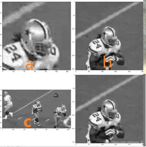
在看这幅图,首先明白 z(1271273) 这里对应着a图,x(2552553)对于的b图,他们都是从图c中以目标为中心,裁剪的一部分
输入搞明白了,在回过头来,从头开始制作数据集,一步步在过一遍。let’go
首先,视频数据集如下,相信很多人会死在这一步,后续,我会整理小的数据集,调试的时候也要用小的数据集。视频教程在制作中…
链接:https://pan.baidu.com/s/1OiW3-cWzsL0FPzjkehyEKg
提取码:3uro
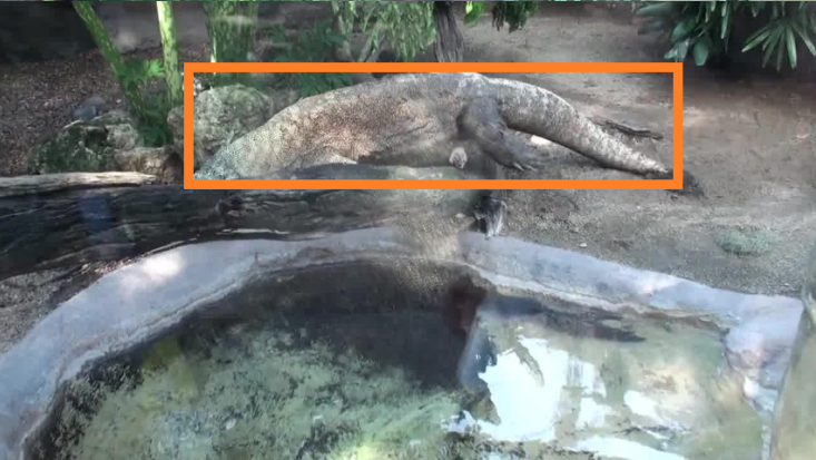
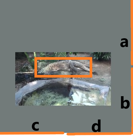
数据集里,由视频中提取图片,通过以下代码,进行转换,得到标有【a,b,c,d】的图,看我标的线段,ab等长,cd 等长,你就会发现没张图的目标恰好在图像中心,这是有意为之。当调试到,标签文件时,你会发现很奇怪,输出是17171的矩阵,标签也是17171,你打印输出可视化时,是黑框橘黄心的那幅图(示意图,之前结果忘保留了,真实图视频再补吧),全标签都是这个,这里也奇怪的,只有一个标签?
在我的构想中,两幅图中,相同部分的值,标签为1,不同为0,标签位置01部分应该实时变化,但是标签位置给固定了,那么就只有一直解释,样本要变,是的输入两个图像要在图像中心相似度最大。 好比我坐在火车上,我看着我的火车走了,实际我的火车对地没有动,那只能是我看的那辆火车走了。这也就解释了图像为何总在中间区域,多出的用全图像素均值填充。这么做,可能编程更容易吧。

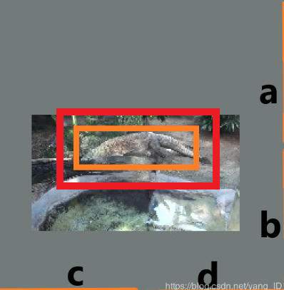
下图的红色区域和橘黄色目标区域,就是孪生网络的两个输入了。这里我们可以多显示几幅图,观察一下,输入数据
import numpy as np
import pickle
import os
import cv2
import functools
import xml.etree.ElementTree as ET
import sys
import argparse
import multiprocessing
from multiprocessing import Pool
# import matplotlib.pyplot as plt # plt 用于显示图片
from fire import Fire
from tqdm import tqdm
from glob import glob
from siamfc import config, get_instance_image

sys.path.append(os.getcwd())

multiprocessing.set_start_method('spawn',True) #开启多线程

def worker(output_dir, video_dir):

    image_names = glob(os.path.join(video_dir, '*.JPEG'))
    # print("................")
    # print("................")
    # print("................")
    #
    # print(image_names)

    #sort函数
    #sorted()作用于任意可以迭代的对象,而sort()一般作用于列表;
    #sort()函数不需要复制原有列表,消耗的内存较少,效率也较高: b=sorted(a)并不改变a的排序,a.sort() 会改变a的排序
    #sorted(classCount.iteritems(),key=operator.itemgetter(1),reverse=True)  #key依据某一列为排序依据
    # image_names = sorted(image_names)
    # print(">>>>>>>>>>>>>>>>>>>>>>>>>")
    # image_names = sorted(image_names,key=lambda x:int(x.split('/')[-1].split('.')[0])) #从小到大进行排列
    #
    # print("<<<<<<<<<<<<<<<<<<<<<")
    # print(image_names)
    video_name = video_dir.split('5\\')[-1]
    # print(">>>>>>>>>>>>>>>>>>>")
    # print(video_name)

    save_folder = os.path.join(output_dir, video_name)
    # print(save_folder)
    # print(save_folder)

    # if not os.path.exists(output_dir):
    #     os.makedirs(output_dir)

    # if not os.path.exists(save_folder):
    #     # print("<<<<<<<<<<<<<<<<<<<<")
    #     os.makedirs(save_folder)
    #     # print("<<<<<<<<<<<222<<<<<<<<<")


    if not os.path.exists(save_folder):
        # print("<<<<<<<<<<<<<<<<<<<<")
        os.makedirs(save_folder)
    # os.makedirs('C:/Users/Administrator/Desktop/SiamFC2/SiamFC-master/bin/data/ILSVRC_VID_CURATION/Data/VID/train/ILSVRC2015_VID_train_0000/ILSVRC2015_train_00000000')
        # print("<<<<<<<<<<<222<<<<<<<<<")


    trajs = {}

    for image_name in image_names:
        img = cv2.imread(image_name)
        #axis=0,表示shape第0个元素被压缩成1,即求每一列的平均值,axis=1,表示输出矩阵是1列(shape第一个元素被压缩成1),求每一行的均值,axis=(0,1)表示shape的第0个元素和第1个元素被压缩成了1
        #元组和列表类似,不同之处在于元组的元素不能修改,元组使用小括号,列表使用方括号,元组的创建很简单,只需要在括号中添加元素,并使用逗号间隔开
        #map(int, img.mean(axis=(0, 1)))将数据全部转换为int类型列表
        img_mean = tuple(map(int, img.mean(axis=(0, 1))))
        anno_name = image_name.replace('Data', 'Annotations') #str.replace('a','b')将str中的a替换为字符串中的b
        anno_name = anno_name.replace('JPEG', 'xml')
        tree = ET.parse(anno_name) #解析xml文件
        root = tree.getroot() #获取根节点; 作为一个元素,root有一个标签和一个属性字典,它也有子节点,for child in root
        bboxes = []
        filename = root.find('filename').text #查找指定标签的文本内容,对于任何标签都可以有三个特征,标签名root.tag,标签属性root.attrib,标签的文本内容root.text
        for obj in root.iter('object'):       #迭代所有的object属性
            bbox = obj.find('bndbox')         #找到objecet中的 boundbox 坐标值
            bbox = list(map(int, [bbox.find('xmin').text,
                                  bbox.find('ymin').text,
                                  bbox.find('xmax').text,
                                  bbox.find('ymax').text]))
            trkid = int(obj.find('trackid').text)
            if trkid in trajs:
                trajs[trkid].append(filename)#如果已经存在,就append
            else:#添加
                trajs[trkid] = [filename]
            #得到目标区域

            instance_img, _, _ = get_instance_image(img, bbox,
                    config.exemplar_size, config.instance_size, config.context_amount, img_mean)

            # plt.imshow(np.array(instance_img))
            # plt.show(instance_img)


            instance_img_name = os.path.join(save_folder, filename+".{:02d}.x.jpg".format(trkid))
            cv2.imwrite(instance_img_name, instance_img)
    return video_name, trajs

def processing(data_dir, output_dir, num_threads=32):
    # get all 4417 videos
    video_dir = os.path.join(data_dir, 'Data\VID') #./data/ILSVRC2015/Data/VID

    #获取训练集和测试集的路径 from glob import glob = glob.glob
    all_videos = glob(os.path.join(video_dir, 'train\ILSVRC2015_VID_train_0000/*')) + \
                 glob(os.path.join(video_dir, 'train\ILSVRC2015_VID_train_0001/*')) + \
                 glob(os.path.join(video_dir, 'train\ILSVRC2015_VID_train_0002/*')) + \
                 glob(os.path.join(video_dir, 'train\ILSVRC2015_VID_train_0003/*')) + \
                 glob(os.path.join(video_dir, 'val/*'))
    #
    # print("==============================")
    # print(all_videos)
    # print("==============================")
    # print(output_dir)
    #all_videos = sorted(all_videos,key=lambda x: int(x.split('/')[-1].split('_')[-1]))
    meta_data = []
    if not os.path.exists(output_dir):
        os.makedirs(output_dir)


    #开启并行运算
        """
        funtional.partial
        可调用的partial对象,使用方法是partial(func,*args,**kw),func是必须要传入的

        imap和imap_unordered都用于对于大量数据遍历的多进程计算
        imap返回结果顺序和输入相同,imap_unordered则为不保证顺序 imap_unordered的返回迭代器的结果的排序是任意的,
        example:
            logging.info(pool.map(fun, range(10))) #把10个数放进函数里面,函数返回一个列表的结果
            pool.imap(fun,range(10))#把10个数放进fun里面,函数返回一个IMapIterator对象,每遍历一次,得到一个结果(进程由操作系统分配)
            pool.imap_unordered(fun,range(10)) #把10个数放进fun,函数返回一个IMapUnorderedIterator对象,每遍历一次得到一个结果

        Pool使用完毕后必须关闭,否则进程不会退出。有两种写法:
        (1)
        iter = pool.imap(func, iter)
        for ret in iter:
            #do something
        (2)推荐
        注意,第二种中,必须在with的块内使用iter
        with Pool() as pool:
            iter = pool.imap(func, iter)
            for ret in iter:
                #do something
        """

    with Pool(processes=num_threads) as pool:
        # print("........................")
        # print(all_videos)
        # print("........................")
        # print(worker)
        # print("........................")
        # print(output_dir)
        functools.partial(worker, output_dir)
        # print("...........=======..........")
        for ret in tqdm(pool.imap_unordered(functools.partial(worker, output_dir), all_videos),
            total=len(all_videos)):
            # print("---------------------")
            meta_data.append(ret) #通过这种方式可以使得进程退出
            # print(ret)

     #开启单线
    # 使用tqdm,一下三种方法都可以使用
    #for num in tqdm(range(0,len(all_videos))):
    #for video in tqdm(all_videos,total=len(all_videos)):
    # for video in tqdm(all_videos):
    #     ret=worker(output_dir, video)
    #     meta_data.append(ret)

    #save meta data
    pickle.dump(meta_data, open(os.path.join(output_dir, "meta_data.pkl"), 'wb'))

Data_dir='./data/ILSVRC2015'
Output_dir='./data/ILSVRC_VID_CURATION'
Num_threads=8# 原来设置为32

if __name__ == '__main__':
    # parse arguments
    parser=argparse.ArgumentParser(description="Demo SiamFC")
    parser.add_argument('--d',default=Data_dir,type=str,help="data_dir")
    parser.add_argument('--o',default=Output_dir,type=str, help="out put")
    parser.add_argument('--t',default=Num_threads, type=int, help="thread_num")
    args=parser.parse_args()

    processing(args.d, args.o, args.t)
    # print("==========end==============")
    #Fire(processing)
    '''
    原来都是使用argparse库进行命令行解析,需要在python文件的开头需要大量的代码设定各个命令行参数。
    而使用fire库不需要在python文件中设定命令行参数的代码,shell中指定函数名和对应参数即可
    train.py
        def train(a,b):
	    return a + b
    第一种调用方法
    train 1 2

    第二种调用方式
    train --a 1 --b 2

    '''
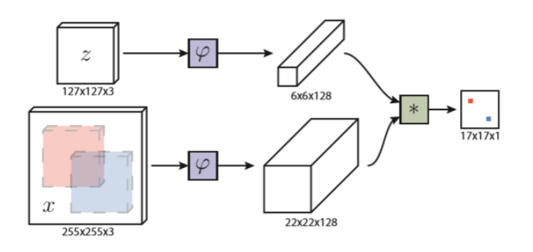
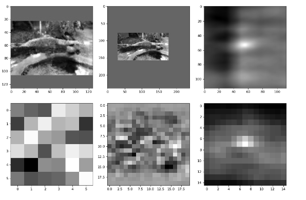
这里输入后, 是AlexNet网络,输出的图 66128 和2222128打印输出一个通道,图如下
 这里是相互卷积,score = F.conv2d(instance, self.exemplar, groups=N),关键代码,就一句,通俗解释一下,就是拿1271273 和2552553,一块块对比,找到相似度最大的一块,通过前面一系列的样本处理,相似度最大的永远在中心区域,对了这里为了解决正负样本不均衡操作,正负样本会给一个系数的
import torch
# import numpy as np
import torch.nn.functional as F
from torch.autograd import Variable
# # import torchvision.transforms as transforms
# # from .custom_transforms import ToTensor
#
# from torchvision.models import alexnet
# from torch.autograd import Variable
import numpy as np
from torch import nn
import matplotlib.pyplot as plt # plt 用于显示图片

from siamfc.config import config

# from .config import config

class SiameseAlexNet(nn.Module):
    def __init__(self, gpu_id, train=True):
        super(SiameseAlexNet, self).__init__()
        self.features = nn.Sequential(
            nn.Conv2d(3, 96, 11, 2),            #(1)Conv1  stride=2 第一个卷积层--输入通道,输出通道,卷积核的大小,(stride)步长
            nn.BatchNorm2d(96),     #输入通道
            nn.ReLU(inplace=True),  #
            nn.MaxPool2d(3, 2),                 #Pool1  stride=2 卷积核大小,stride步长
            nn.Conv2d(96, 256, 5, 1, groups=2), #(2)Conv2  stride=2    对于每一个组输入是48 第二个卷积层
            nn.BatchNorm2d(256),  #输入通道,
            nn.ReLU(inplace=True),
            nn.MaxPool2d(3, 2),                 #Pool2 stride=2
            nn.Conv2d(256, 384, 3, 1),          #(3)Conv3
            nn.BatchNorm2d(384),
            nn.ReLU(inplace=True),
            nn.Conv2d(384, 384, 3, 1, groups=2),#(4)Conv4 groups分成两个组,对于每一个组输入是192
            nn.BatchNorm2d(384),
            nn.ReLU(inplace=True),
            nn.Conv2d(384, 256, 3, 1, groups=2) #(5)Conv5
        )
        self.corr_bias = nn.Parameter(torch.zeros(1)) # Parameter

        """
        ==============================================================
        输出是 1*1**15*15
        这里是为了和统一格式输出
        F.binary_cross_entropy_with_logits(pred, target, weights, reduction = reduction)
        weights 解决分割任务会遇到正负样本不均的问题

        ==============================================================
        """
        if train:  # 下杠+函数名 警告是私有函数,但是外部依然可以调用  train_response_sz=15  训练阶段的响应图 15x15
            gt, weight = self._create_gt_mask((config.train_response_sz, config.train_response_sz))


            # print("==============================")
            # print("==============================")
            # print("==============================")
            # print("==============================")
            # print(gt)

            # print(config.train_response_sz)

            #数据类型转换
            with torch.cuda.device(gpu_id):
                self.train_gt = torch.from_numpy(gt).cuda()
                self.train_weight = torch.from_numpy(weight).cuda() #train_gt.dtype=torch.float32
            gt, weight = self._create_gt_mask((config.response_sz, config.response_sz)) #response_sz=17 验证阶段的响应图 17x17
            with torch.cuda.device(gpu_id): #验证集 17x17
                self.valid_gt = torch.from_numpy(gt).cuda()
                self.valid_weight = torch.from_numpy(weight).cuda()
        self.exemplar = None #范例
        self.gpu_id = gpu_id

    ''' self.modules() ,self.children() https://blog.csdn.net/dss_dssssd/article/details/83958518
        modules 包含了网络的本身和所有的子模块(深度优先遍历)  children只包含了第二层的网络
    '''
    def init_weights(self):
        for m in self.modules(): #第一次返回的是网络本身 m=SiameseAlexNet
            '''
             #关于isinstance和type的比较 https://www.runoob.com/python/python-func-isinstance.html
             type不会认为子类是一种父类类型,不考虑继承关系.
             isinstance 会认为子类是一种父类类型,会考虑继承关系
            '''
            if isinstance(m, nn.Conv2d): # fan_in 保持weights的方差在前向传播中不变,使用fan_out保持weights的方差在反向传播中不必变
                nn.init.kaiming_normal_(m.weight.data, mode='fan_out', nonlinearity='relu')#正态分布
            elif isinstance(m, nn.BatchNorm2d):
                m.weight.data.fill_(1)   # pytorch中,一般来说,如果对tensor的一个函数后加上了下划线,则表明这是一个in-place类型
                m.bias.data.zero_()      # app

    def forward(self, x):
        exemplar, instance = x  # x = ( exemplar, instance )
        # 训 练 阶 段
        if exemplar is not None and instance is not None:#
            print(instance.shape)
            print(exemplar.shape)
            print("-------11111111111--------")
            batch_size = exemplar.shape[0] #
            plt.figure(figsize=(16,16), dpi=80)
            plt.figure(1)
            ax1 = plt.subplot(441)
            plt.imshow(exemplar[0,0].cuda().data.cpu().numpy(),cmap='gray')
            ax1 = plt.subplot(442)
            plt.imshow(instance[0,0].cuda().data.cpu().numpy(),cmap='gray')
            # plt.show()

            N, C, H, W = instance.shape
            instance = instance.view(1, -1, H, W)
            score2 = F.conv2d(instance, exemplar, groups=N) * config.response_scale + self.corr_bias
            ax1 = plt.subplot(443)
            plt.imshow(score2[0,0].cuda().data.cpu().numpy(),cmap='gray')

            exemplar = self.features(exemplar) # 8 ,256, 6 , 6
            instance = self.features(instance) # 8,  256, 20, 20

            ax1 = plt.subplot(445)
            plt.imshow(exemplar[0,0].cuda().data.cpu().numpy(),cmap='gray')
            # plt.show()
            ax1 = plt.subplot(446)
            plt.imshow(instance[0,0].cuda().data.cpu().numpy(),cmap='gray')
            # plt.show()


            score_map = []
            N, C, H, W = instance.shape
            instance = instance.view(1, -1, H, W)

            #互卷积
            score = F.conv2d(instance, exemplar, groups=N) * config.response_scale + self.corr_bias
            print("-------------------------")
            print("-------------------------")
            """
            ============================================
            instance[1, 256, 20, 20]   torch.Size([1, 3, 239, 239])
            exemplar([1, 256, 6, 6])   ([1, 3, 127, 127])

            score  [1, 1, 15, 15]


            ============================================

            """
            # print(score.shape)
            # print(instance.shape)
            # print(exemplar.shape)
            ax1 = plt.subplot(447)
            plt.imshow(score[0,0].cuda().data.cpu().numpy(),cmap='gray')
            plt.show()

            # print(score)
            return score.transpose(0, 1) # 0和1维度交换
        # 测 试 阶 段(第一帧初始化)


        elif exemplar is not None and instance is None: #初始化的时候只输入了exemplar
            print("-------22222222222--------")
            # inference used 提取模板特征
            self.exemplar = self.features(exemplar) #1,256, 6, 6
            self.exemplar = torch.cat([self.exemplar for _ in range(3)], dim=0) # [3,256,6,6]
        # 测 试 阶 段 (非第一帧)
        else:
            print("-------3333333333333--------")
            # inference used we don't need to scale the response or add bias
            instance = self.features(instance)  #提取搜索区域的特征,包含三个尺度
            N, _, H, W = instance.shape

            print(instance.shape)
            instance = instance.view(1, -1, H, W) # 1,NxC,H, W
            score = F.conv2d(instance, self.exemplar, groups=N)
            return score.transpose(0, 1)

    def loss(self, pred):
        return F.binary_cross_entropy_with_logits(pred, self.gt)

    # input = torch.randn(3, requires_grad=True)
    # target = torch.empty(3).random_(2)
    # loss = F.binary_cross_entropy_with_logits(input, target)
    # loss.backward()
    def weighted_loss(self, pred):
        if self.training:
            # print("--------------------------------------")
            # print("--------------------------------------")
            # print(self.train_gt)


            return F.binary_cross_entropy_with_logits(pred, self.train_gt,
                    self.train_weight, reduction='sum') / config.train_batch_size # normalize the batch_size
        else:
            # print("++++++++++++444444444444443++++++++++++++++++")
            return F.binary_cross_entropy_with_logits(pred, self.valid_gt,
                    self.valid_weight, reduction='sum') / config.valid_batch_size # normalize the batch_size
    #生成样本的标签和标签的权重
    def _create_gt_mask(self, shape):
        # same for all pairs
        h, w = shape                                     # shape=[15,15]  255x255对应17x17   (255-2*8)x(255-2*8) 对应 15x15
        y = np.arange(h, dtype=np.float32) - (h-1) / 2.  # [0,1,2...,14]-(15-1)/2-->y=[-7, -6 ,...0,...,6,7]
        x = np.arange(w, dtype=np.float32) - (w-1) / 2.  # [0,1,2...,14]-(15-1)/2-->x=[-7, -6 ,...0,...,6,7]
        y, x = np.meshgrid(y, x)                          #生成格点,将图划分成小块
        # print("...............")
        # print(y)
        dist = np.sqrt(x**2 + y**2)                      # ||u-c|| 代表到中心点的距离
        mask = np.zeros((h, w))
        mask[dist <= config.radius / config.total_stride] = 1 # ||u-c||×total_stride <= radius  距离小于radius的位置是1
        plt.imshow(mask)
        plt.show()
        mask = mask[np.newaxis, :, :]                         # np.newaxis 意思是在这一个维度再增加一个一维度 mask.shape=(1,15,15)
        weights = np.ones_like(mask)  #np.ones_like 生成一个全是1的和mask一样维度

        #给正负样本配备一个系数,解决正负样本不均衡问题
        weights[mask == 1] = 0.5 / np.sum(mask == 1)   # 0.5/num(positive sample)
        weights[mask == 0] = 0.5 / np.sum(mask == 0)   # 0.5/num(negative sample)

        mask = np.repeat(mask, config.train_batch_size, axis=0)[:, np.newaxis, :, :]#np.repeat(mask,batch,axis=0)数组重复三次
        return mask.astype(np.float32), weights.astype(np.float32) # mask.shape=(8,1,15,15) train_num_workers=0的情况

# print("==========")

#
#
# import numpy as np
# import matplotlib.pyplot as plt # plt 用于显示图片
#
# exemplar_imgs_numpy=np.load("exemplar_imgs_numpy3.npy")[0:1]
# instance_imgs_numpy=np.load("instance_imgs_numpy3.npy")[0:1]
# exemplar_imgs=torch.from_numpy(exemplar_imgs_numpy).float()
# instance_imgs=torch.from_numpy(instance_imgs_numpy).float()
#
#
# """
# ==================================================
# exemplar_imgs 127*127
# instance_imgs 239*239
# ==================================================
# """
# print(exemplar_imgs.shape)
# print(instance_imgs.shape)
#
# model = SiameseAlexNet('cuda', train=True) #__init__
# # model.init_weights() #init_weights 主要是卷积层和归一化层参数初始化
# # model.train() #设置模型为训练模式
# # print(model)
# model.init_weights()
# model.cuda()
# model.train()
#
# exemplar_var, instance_var = Variable(exemplar_imgs.cuda()), Variable(instance_imgs.cuda()) # 这两个必须是Variable吗
# # # print(exemplar_var)
# # # optimizer.zero_grad() # 梯度清零
# # # print("===========model=============")
# outputs = model((exemplar_var, instance_var)) # [8, 1, 15, 15]
#
# print(outputs.shape)
# loss = model.weighted_loss(outputs) # loss是tensor
#
#
#
#
#


# # print("===========loss=============")
# loss.backward()
# optimizer.step() # 梯度参数更新


# print(exemplar_imgs_numpy.shape)
# print(instance_imgs_numpy.shape)
# exemplar_imgs_show=exemplar_imgs_numpy
# instance_imgs_show=instance_imgs_numpy
# # print(exemplar_imgs_numpy.shape)
# # print(instance_imgs_numpy.shape)
# #
# exemplar_imgs_show=(exemplar_imgs_show-np.min(exemplar_imgs_show))/(np.max(exemplar_imgs_show)-np.min(exemplar_imgs_show))
# instance_imgs_show=(instance_imgs_show-np.min(instance_imgs_show))/(np.max(instance_imgs_show)-np.min(instance_imgs_show))
#
#
# plt.figure(figsize=(16,16), dpi=80)
# plt.figure(1)
# ax1 = plt.subplot(441)
# plt.imshow(instance_imgs_show[1,0,:,:],cmap='gray')
# ax1 = plt.subplot(442)
# plt.imshow(exemplar_imgs_show[1,0,:,:],cmap='gray')
#
# ax1 = plt.subplot(443)
# plt.imshow(instance_imgs_show[2,0,:,:],cmap='gray')
# ax1 = plt.subplot(444)
# plt.imshow(exemplar_imgs_show[2,0,:,:],cmap='gray')
#
# ax1 = plt.subplot(445)
# plt.imshow(instance_imgs_show[3,0,:,:],cmap='gray')
# ax1 = plt.subplot(446)
# plt.imshow(exemplar_imgs_show[3,0,:,:],cmap='gray')
#
#
# ax1 = plt.subplot(447)
# plt.imshow(instance_imgs_show[4,0,:,:],cmap='gray')
# ax1 = plt.subplot(448)
# plt.imshow(exemplar_imgs_show[4,0,:,:],cmap='gray')
#
#
# ax1 = plt.subplot(449)
# plt.imshow(instance_imgs_show[5,0,:,:],cmap='gray')
# ax1 = plt.subplot(4,4,10)
# plt.imshow(exemplar_imgs_show[5,0,:,:],cmap='gray')
#
# ax1 = plt.subplot(4,4,11)
# plt.imshow(instance_imgs_show[6,0,:,:],cmap='gray')
# ax1 = plt.subplot(4,4,12)
# plt.imshow(exemplar_imgs_show[6,0,:,:],cmap='gray')
#
# ax1 = plt.subplot(4,4,13)
# plt.imshow(instance_imgs_show[7,0,:,:],cmap='gray')
# ax1 = plt.subplot(4,4,14)
# plt.imshow(exemplar_imgs_show[7,0,:,:],cmap='gray')
#
# ax1 = plt.subplot(4,4,15)
# plt.imshow(instance_imgs_show[8,0,:,:],cmap='gray')
# ax1 = plt.subplot(4,4,16)
# plt.imshow(exemplar_imgs_show[8,0,:,:],cmap='gray')
#
# plt.show()
单目标跟踪
bilibili演示视频 https://www.bilibili.com/video/BV1FZ4y1M7NL/
siamfc单目标检测
siamfc单目标检测2
这里是以下代码的展示效果,
通过孪生网络,可以得到目标物的移动方向,仔细观看视频,移动后可以得到相对位移,然后是位置变动的坐标,通过位置变动的坐标跟新输入孪生网络区域,在进行位置跟新,一旦目标物跟丢,就很难找到目标物
import numpy as np
import cv2
import torch
import torch.nn.functional as F
import time
import warnings
import torchvision.transforms as transforms

from torch.autograd import Variable
import matplotlib.pyplot as plt # plt 用于显示图片
from .alexnet import SiameseAlexNet
from .config import config
from .custom_transforms import ToTensor
from .utils import get_exemplar_image, get_pyramid_instance_image, get_instance_image

torch.set_num_threads(1) # otherwise pytorch will take all cpus

class SiamFCTracker:
    def __init__(self, model_path, gpu_id):
        self.gpu_id = gpu_id
        with torch.cuda.device(gpu_id):
            self.model = SiameseAlexNet(gpu_id, train=False)
            self.model.load_state_dict(torch.load(model_path))
            self.model = self.model.cuda()
            self.model.eval()
        self.transforms = transforms.Compose([
            ToTensor()
        ])

    def _cosine_window(self, size):
        """
            get the cosine window
        """
        print("----------cosine---------------")
        print(np.array(size).shape)
        cos_window = np.hanning(int(size[0]))[:, np.newaxis].dot(np.hanning(int(size[1]))[np.newaxis, :])
        cos_window = cos_window.astype(np.float32)
        cos_window /= np.sum(cos_window)
        print(np.array(cos_window).shape)
        return cos_window

    def init(self, frame, bbox):
        """ initialize siamfc tracker
        Args:
            frame: an RGB image
            bbox: one-based bounding box [x, y, width, height]
        """
        self.bbox = (bbox[0]-1, bbox[1]-1, bbox[0]-1+bbox[2], bbox[1]-1+bbox[3]) # zero based

        #这里是变化的
        self.pos = np.array([bbox[0]-1+(bbox[2]-1)/2, bbox[1]-1+(bbox[3]-1)/2])  # center x, center y, zero based
        self.target_sz = np.array([bbox[2], bbox[3]])                            # width, height
        # get exemplar img
        self.img_mean = tuple(map(int, frame.mean(axis=(0, 1))))
        exemplar_img, scale_z, s_z = get_exemplar_image(frame, self.bbox,
                config.exemplar_size, config.context_amount, self.img_mean)


        # print("exemplar_img:",np.array(exemplar_img).shape)
        #
        # #得到需要搜索的图像
        # plt.figure(figsize=(16, 16), dpi=80)
        # plt.figure(1)
        # ax1 = plt.subplot(221)
        # plt.imshow(np.array(exemplar_img)[:,:,0], cmap='gray')


        # get exemplar feature
        exemplar_img = self.transforms(exemplar_img)[None,:,:,:]


        print("exemplar_img:", np.array(exemplar_img).shape)
        #变为GPU 变量
        with torch.cuda.device(self.gpu_id):
            exemplar_img_var = Variable(exemplar_img.cuda())
            self.model((exemplar_img_var, None))

        self.penalty = np.ones((config.num_scale)) * config.scale_penalty
        self.penalty[config.num_scale//2] = 1


        # create cosine window  上采样 stride=2^4=16, 响应图的大小 17x17
        self.interp_response_sz = config.response_up_stride * config.response_sz
        self.cosine_window = self._cosine_window((self.interp_response_sz, self.interp_response_sz))


        # create scalse
        # scale_z  # s-x原始 “搜索区域”的大小;s-z是原始模板的大小
        self.scales = config.scale_step ** np.arange(np.ceil(config.num_scale/2)-config.num_scale,
                np.floor(config.num_scale/2)+1)

        print("==============================================")
        print(self.scales)
        print("==============================================")


        # create s_x
        self.s_x = s_z + (config.instance_size-config.exemplar_size) / scale_z

        # arbitrary scale saturation
        self.min_s_x = 0.2 * self.s_x  ##搜索区域下限=原始的搜索区域的1/5
        self.max_s_x = 5 * self.s_x   #搜索区域上限=原始的搜索区域的5倍

    def update(self, frame):
        """track object based on the previous frame
        Args:
            frame: an RGB image

        Returns:
            bbox: tuple of 1-based bounding box(xmin, ymin, xmax, ymax)
        """
        size_x_scales = self.s_x * self.scales
        print("=================================")
        print(size_x_scales)
        print("pose:",self.pos)
        print(config.instance_size)
        print("=================================")

        """
        ========================================
        self.bbox = (bbox[0]-1, bbox[1]-1, bbox[0]-1+bbox[2], bbox[1]-1+bbox[3]) # zero based
        self.pos = np.array([bbox[0]-1+(bbox[2]-1)/2, bbox[1]-1+(bbox[3]-1)/2])  # center x, center y, zero based
        中心点坐标

        pos: [316.10938432 113.95910831]   这里也是变化的

        config.instance_size  跟踪用的初步窗口大小【255,255】

        size_x_scales = self.s_x * self.scales  位置移动  [171.91251587 178.35923522 185.04770654]


        self.img_mean  平均值填充

        pyramid  (3, 255, 255, 3)

        ========================================
        """


        pyramid = get_pyramid_instance_image(frame, self.pos, config.instance_size, size_x_scales, self.img_mean)


        print("pyramid:",np.array(pyramid).shape)
        # print("______________pr______________________")
        # print('fram:',np.array(frame).shape)
        # print('pyramid:',np.array(pyramid).shape)
        # plt.figure(figsize=(16, 16), dpi=80)
        # plt.figure(1)
        # ax1 = plt.subplot(222)
        # plt.imshow(np.array(pyramid)[0,:,:,0], cmap='gray')
        # plt.figure(1)
        # ax1 = plt.subplot(223)
        # plt.imshow(np.array(frame[:,:,0]), cmap='gray')
        # # plt.imshow(exemplar[0, 0].cuda().data.cpu().numpy(), cmap='gray')


        #数据转换
        instance_imgs = torch.cat([self.transforms(x)[None,:,:,:] for x in pyramid], dim=0)

        #
        # ax1 = plt.subplot(224)
        # print(np.array(instance_imgs).shape)
        # plt.imshow(np.array(instance_imgs[0,0,:,:]), cmap='gray')
        # # plt.imshow(exemplar[0, 0].cuda().data.cpu().numpy(), cmap='gray')
        # plt.show()


        with torch.cuda.device(self.gpu_id):
            instance_imgs_var = Variable(instance_imgs.cuda())

            response_maps = self.model((None, instance_imgs_var))
            response_maps = response_maps.data.cpu().numpy().squeeze()
            #上采样
            response_maps_up = [cv2.resize(x, (self.interp_response_sz, self.interp_response_sz), cv2.INTER_CUBIC)
             for x in response_maps]

            #response_maps: (3, 17, 17)
            #response_maps_up: (3, 272, 272)

            # print("response_maps:", response_maps.shape)
            # print("response_maps_up:",np.array(response_maps_up).shape)
        # plt.figure(figsize=(16, 16), dpi=80)
        # plt.figure(1)
        # ax1 = plt.subplot(221)
        # plt.imshow(np.array(response_maps[0,:,:]), cmap='gray')
        # plt.show()


        # get max score  找到目标位置
        max_score = np.array([x.max() for x in response_maps_up]) * self.penalty


        # penalty scale change
        scale_idx = max_score.argmax()
        response_map = response_maps_up[scale_idx]#找到最大响应尺度对应的最大响应图
        ax1 = plt.subplot(222)
        # plt.imshow(np.array(response_maps[0,:,:]), cmap='gray')

        response_map -= response_map.min() #响应值减去最小值
        ax1 = plt.subplot(223)
        # plt.imshow(np.array(response_maps[0,:,:]), cmap='gray')

        response_map /= response_map.sum()  #归一化

        response_map = (1 - config.window_influence) * response_map + \
                config.window_influence * self.cosine_window  #添加余弦窗

        # ax1 = plt.subplot(224)
        # plt.imshow(np.array(response_maps[0, :, :]), cmap='gray')
        # plt.show()
        #


        max_r, max_c = np.unravel_index(response_map.argmax(), response_map.shape)  #获取索引值在response-map中的位置
        # displacement in interpolation response 插值响应中的位移,相对于中心点的位移
        disp_response_interp = np.array([max_c, max_r]) - (self.interp_response_sz-1) / 2.

        # displacement in input
        disp_response_input = disp_response_interp * config.total_stride / config.response_up_stride
        # displacement in frame
        """"
        中间点的相对位移
        disp_response_interp
        [-0.5 -0.5]
         [-15.5 -15.5]
         [0.5 0.5]

         disp_response_input  位移长度原图的还原
        """
        print("disp_response_interp:", disp_response_interp)

        scale = self.scales[scale_idx]
        disp_response_frame = disp_response_input * (self.s_x * scale) / config.instance_size
        # position in frame coordinates
        self.pos += disp_response_frame

        #变化位移的坐标


        # scale damping and saturation
        self.s_x *= ((1 - config.scale_lr) + config.scale_lr * scale)
        self.s_x = max(self.min_s_x, min(self.max_s_x, self.s_x))
        self.target_sz = ((1 - config.scale_lr) + config.scale_lr * scale) * self.target_sz
        bbox = (self.pos[0] - self.target_sz[0]/2 + 1, # xmin   convert to 1-based
                self.pos[1] - self.target_sz[1]/2 + 1, # ymin
                self.pos[0] + self.target_sz[0]/2 + 1, # xmax
                self.pos[1] + self.target_sz[1]/2 + 1) # ymax
        return bbox
发布者:全栈程序员-站长,转载请注明出处:https://javaforall.net/186951.html原文链接:https://javaforall.net


