
R语言基础画图
R语言免费且开源,其强大和自由的画图功能,深受广大学生和可视化工作人员喜爱,这篇文章对如何使用R语言作基本的图形,如直方图,点图,饼状图以及箱线图进行简单介绍。
0 结构
1 点图
点图,简单的讲就是每个数据点按照其对应的横纵坐标位置对应在坐标系中的图形,什么是点图就不做过多介绍了。
- 点图标准代码:
dotchart(x, labels = NULL, groups = NULL, gdata = NULL, cex = par("cex"), pt.cex = cex, pch = 21, gpch = 21, bg = par("bg"), color = par("fg"), gcolor = par("fg"), lcolor = "gray", xlim = range(x[is.finite(x)]), main = NULL, xlab = NULL, ylab = NULL, ...) dotchart(mtcars$mpg,labels = row.names(mtcars),cex = .7, main = "Gas Mileage for Car Models", xlab = "Miles Per gallon") 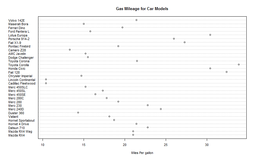

散点图1.1
x <- mtcars[order(mtcars$mpg),] #按照mpg排序 x$cyl <-factor(x$cyl) #将cyl变成因子数据结构类型 x$color[x$cyl==4] <-"red" #新建一个color变量,油缸数cyl不同,颜色不同 x$color[x$cyl==6] <-"blue" x$color[x$cyl==8] <-"darkgreen" dotchart(x$mpg, #数据对象 labels = row.names(x), #标签 cex = .7,#字体大小 groups = x$cyl, #按照cyl分组 gcolor = "black", #分组颜色 color = x$color, #数据点颜色 pch = 19,#点类型 main = "Gas Mileage for car modes \n grouped by cylinder", #标题 xlab = "miles per gallon") #x轴标签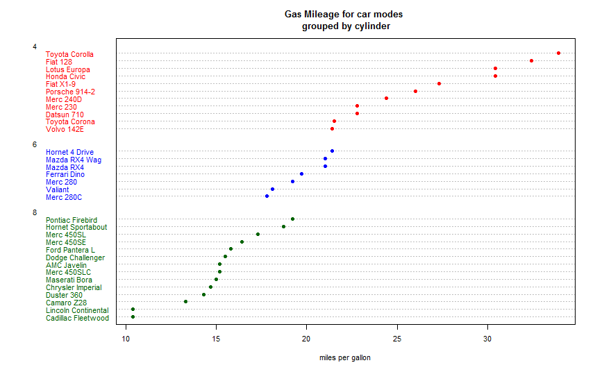
散点图1.2
是不是好看多了,嘻嘻!按照油缸数不同进行了分类,并且可以看出油缸数量越多越耗油。
2 直方图
2.1 直方图
小学生都知道的条形图,怎么弄?
- 条形图标准代码:
barplot(height, ...)是太简单了吗?这么粗暴,就给了一个变量。
- 实例
eg2.1.1
library(vcd) counts <- table(Arthritis$Improved) #引入vcd包只是想要Arthritis中的数据 barplot(counts,main = "bar plot",xlab = "improved",ylab = "counts")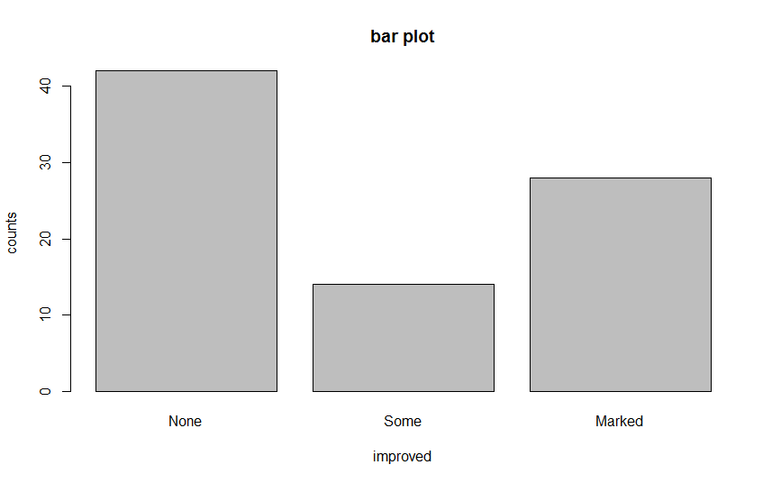
条形图2.1.1
eg2.1.2
barplot(counts,main = " horizontal bar plot", xlab = "frequency", ylab = "improved", horiz = TRUE)#horizon 值默认是FALSE,为TRUE的时候表示图形变为水平的
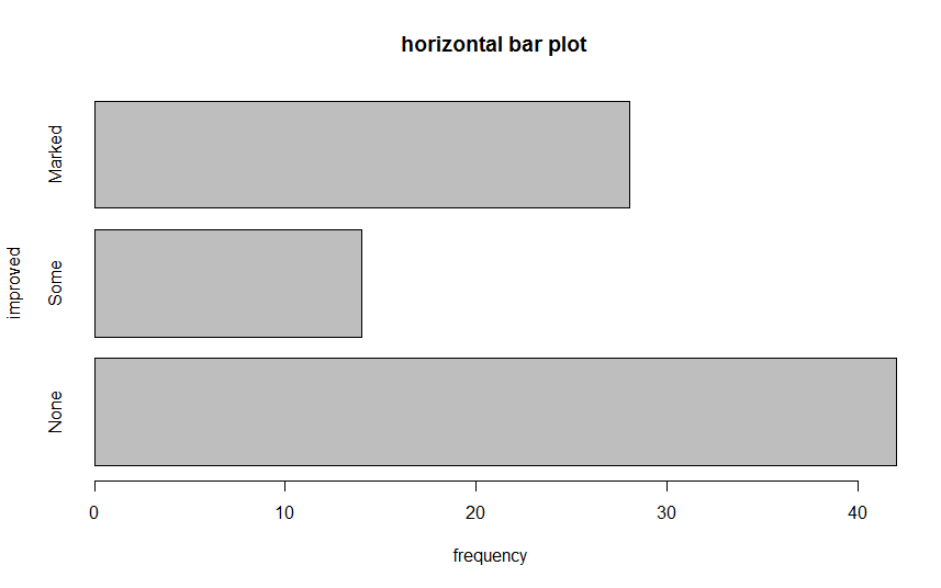
条形图2.1.2
install.packages("vcd") library(vcd) counts <- table(Arthritis$Improved,Arthritis$Treatment) counts数据如下所示:
| Placebo | Treated |
|---|---|
| None | 29 |
| Some | 7 |
| Marked | 7 |
barplot(counts,main = " stacked bar plot",xlab = "treated",ylab = "frequency", col = c("red","yellow","green"), #设置颜色 legend = rownames(counts)) #设置图例
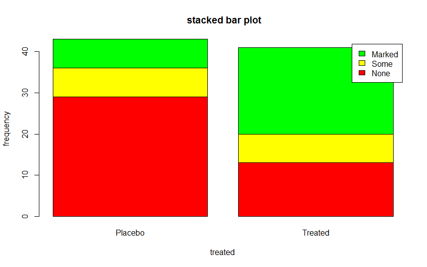
2.1.3.1堆砌条形图
- 代码
eg2.1.3.2
barplot(counts,main = " grouped bar plot",xlab = "treated",ylab = "frequency", col = c("red","yellow","green"), legend = rownames(counts),beside = TRUE)
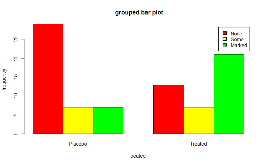
分组条形图2.1.3.2
请注意,两幅图的区别在于2.1.3.2设置了beside = TRUE,beside默认值是FALSE,绘图结果是堆砌条形图,beside值为TRUE时,结果是分组条形图。
2.2荆棘图
library(vcd) attach(Arthritis) counts <- table (Treatment,Improved) spine(counts,main = "Spinogram Example") detach(Arthritis)
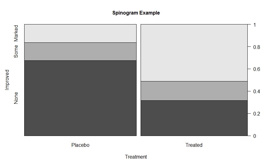
荆棘图2.2
3 直方图
- 直方图标准代码:
hist(x, ...)par (mfrow = c(2,2)) #设置四幅图片一起显示 hist(mtcars$mpg) #基本直方图 hist(mtcars$mpg, breaks = 12, #指定组数 col= "red", #指定颜色 xlab = "Miles per Gallon", main = "colored histogram with 12 bins") hist(mtcars$mpg, freq = FALSE, #表示不按照频数绘图 breaks = 12, col = "red", xlab = "Miles per Gallon", main = "Histogram,rug plot,density curve") rug(jitter(mtcars$mpg)) #添加轴须图 lines(density(mtcars$mpg),col= "blue",lwd=2) #添加密度曲线 x <-mtcars$mpg h <-hist(x,breaks = 12, col = "red", xlab = "Miles per Gallon", main = "Histogram with normal and box") xfit <- seq(min(x),max(x),length=40) yfit <-dnorm(xfit,mean = mean(x),sd=sd(x)) yfit <- yfit *diff(h$mids[1:2])*length(x) lines(xfit,yfit,col="blue",lwd=2) #添加正太分布密度曲线 box() #添加方框
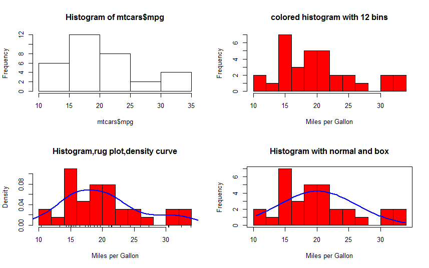
直方图3.1
4 饼图
- 标准饼图代码:
pie(x, labels = names(x), edges = 200, radius = 0.8, clockwise = FALSE, init.angle = if(clockwise) 90 else 0, density = NULL, angle = 45, col = NULL, border = NULL, lty = NULL, main = NULL, ...)- 实例
eg4.1
par(mfrow = c(2,2)) slices <- c(10,12,4,16,8) #数据 lbls <- c("US","UK","Australis","Germany","France") #标签数据 pie(slices,lbls) #基本饼图 pct <- round(slices/sum(slices)*100) #数据比例 lbls2 <- paste(lbls," ",pct ,"%",sep = "") pie(slices,labels = lbls2,col = rainbow(length(lbls2)), #rainbow是一个彩虹色调色板 main = "Pie Chart with Percentages") library(plotrix) pie3D(slices,labels=lbls,explode=0.1,main="3D pie chart") #三维饼图 mytable <- table (state.region) lbls3 <- paste(names(mytable),"\n",mytable,sep = "") pie(mytable,labels = lbls3, main = "pie chart from a table \n (with sample sizes")
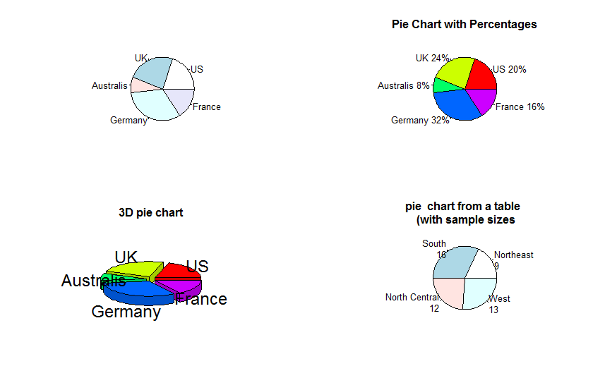
4.1 饼状图
5 箱线图
5.1 箱线图
- 标准箱线图代码:
boxplot(x, ...)- 实例
eg5.1
boxplot(mtcars$mpg,main="Box plot",ylab ="Miles per Gallon") #标准箱线图 boxplot(mpg ~ cyl,data= mtcars, main="car milesge data", xlab= "Number of cylinders", ylab= "Miles per Gallon") boxplot(mpg ~ cyl,data= mtcars, notch=TRUE, #含有凹槽的箱线图 varwidth = TRUE, #宽度和样本大小成正比 col= "red", main="car milesge data", xlab= "Number of cylinders", ylab= "Miles per Gallon") mtcars$cyl.f<- factor(mtcars$cyl, #转换成因子结构 levels= c(4,6,8), labels = c("4","6","8")) mtcars$am.f <- factor(mtcars$am,levels = c(0,1), labels = c("auto","standard")) boxplot(mpg~ am.f*cyl.f, #分组的箱线图 data = mtcars, varwidth=TRUE, col= c("gold","darkgreen"), main= "MPG Distribution by Auto Type", xlab="Auto Type", ylxb="Miles per Gallon")
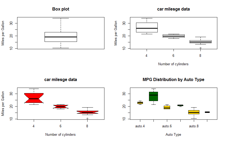
5.1 箱线图
5.2 小提琴图
小提琴图是箱线图和密度图的结合。使用vioplot包中的vioplot函数进行绘图。
- 小提琴图标准代码:
vioplot( x, ..., range=1.5, h, ylim, names, horizontal=FALSE, col="magenta", border="black", lty=1, lwd=1, rectCol="black", colMed="white", pchMed=19, at, add=FALSE, wex=1, drawRect=TRUE)- 实例
代码:
eg5.2
library(vioplot) x1 <- mtcars$mpg[mtcars$cyl==4] x2 <- mtcars$mpg[mtcars$cyl==6] x3 <- mtcars$mpg[mtcars$cyl==8] vioplot(x1,x2,x3,names= c("4 cyl","6 cyl","8 cyl"),col = "gold") title(main="Violin plots of Miles Per Gallon",xlab = "number of cylinders",ylab = "Miles per gallon")白点是中位数,中间细线表示须,粗线对应上下四分位点,外部形状是其分布核密度。
版权声明:本文内容由互联网用户自发贡献,该文观点仅代表作者本人。本站仅提供信息存储空间服务,不拥有所有权,不承担相关法律责任。如发现本站有涉嫌侵权/违法违规的内容, 请联系我们举报,一经查实,本站将立刻删除。
发布者:全栈程序员-站长,转载请注明出处:https://javaforall.net/200360.html原文链接:https://javaforall.net


