
import pandas as pd import numpy as np import math from matplotlib import pyplot as plt from matplotlib.pylab import mpl import tensorflow as tf from sklearn.preprocessing import MinMaxScaler from keras import backend as K from keras.layers import LeakyReLU from tcn import TCN,tcn_full_summary from sklearn.metrics import mean_squared_error # 均方误差 from keras.callbacks import LearningRateScheduler from keras.callbacks import EarlyStopping from tensorflow.keras import Input, Model,Sequential mpl.rcParams['font.sans-serif'] = ['SimHei'] #显示中文 mpl.rcParams['axes.unicode_minus']=False #显示负号 取数据
data=pd.read_csv('mock_kaggle.csv',encoding ='gbk',parse_dates=['datetime']) Date=pd.to_datetime(data.datetime) data['date'] = Date.map(lambda x: x.strftime('%Y-%m-%d')) datanew=data.set_index(Date) series = pd.Series(datanew['股票'].values, index=datanew['date']) series date 2014-01-01 4972 2014-01-02 4902 2014-01-03 4843 2014-01-04 4750 2014-01-05 4654 ... 2016-07-27 3179 2016-07-28 3071 2016-07-29 4095 2016-07-30 3825 2016-07-31 3642 Length: 937, dtype: int64 滞后扩充数据
dataframe1 = pd.DataFrame() num_hour = 16 for i in range(num_hour,0,-1): dataframe1['t-'+str(i)] = series.shift(i) dataframe1['t'] = series.values dataframe3=dataframe1.dropna() dataframe3.index=range(len(dataframe3)) dataframe3 | t-16 | t-15 | t-14 | t-13 | t-12 | t-11 | t-10 | t-9 | t-8 | t-7 | t-6 | t-5 | t-4 | t-3 | t-2 | t-1 | t | |
|---|---|---|---|---|---|---|---|---|---|---|---|---|---|---|---|---|---|
| 0 | 4972.0 | 4902.0 | 4843.0 | 4750.0 | 4654.0 | 4509.0 | 4329.0 | 4104.0 | 4459.0 | 5043.0 | 5239.0 | 5118.0 | 4984.0 | 4904.0 | 4822.0 | 4728.0 | 4464 |
| 1 | 4902.0 | 4843.0 | 4750.0 | 4654.0 | 4509.0 | 4329.0 | 4104.0 | 4459.0 | 5043.0 | 5239.0 | 5118.0 | 4984.0 | 4904.0 | 4822.0 | 4728.0 | 4464.0 | 4265 |
| 2 | 4843.0 | 4750.0 | 4654.0 | 4509.0 | 4329.0 | 4104.0 | 4459.0 | 5043.0 | 5239.0 | 5118.0 | 4984.0 | 4904.0 | 4822.0 | 4728.0 | 4464.0 | 4265.0 | 4161 |
| 3 | 4750.0 | 4654.0 | 4509.0 | 4329.0 | 4104.0 | 4459.0 | 5043.0 | 5239.0 | 5118.0 | 4984.0 | 4904.0 | 4822.0 | 4728.0 | 4464.0 | 4265.0 | 4161.0 | 4091 |
| 4 | 4654.0 | 4509.0 | 4329.0 | 4104.0 | 4459.0 | 5043.0 | 5239.0 | 5118.0 | 4984.0 | 4904.0 | 4822.0 | 4728.0 | 4464.0 | 4265.0 | 4161.0 | 4091.0 | 3964 |
| … | … | … | … | … | … | … | … | … | … | … | … | … | … | … | … | … | … |
| 916 | 1939.0 | 1967.0 | 1670.0 | 1532.0 | 1343.0 | 1022.0 | 813.0 | 1420.0 | 1359.0 | 1075.0 | 1015.0 | 917.0 | 1550.0 | 1420.0 | 1358.0 | 2893.0 | 3179 |
| 917 | 1967.0 | 1670.0 | 1532.0 | 1343.0 | 1022.0 | 813.0 | 1420.0 | 1359.0 | 1075.0 | 1015.0 | 917.0 | 1550.0 | 1420.0 | 1358.0 | 2893.0 | 3179.0 | 3071 |
| 918 | 1670.0 | 1532.0 | 1343.0 | 1022.0 | 813.0 | 1420.0 | 1359.0 | 1075.0 | 1015.0 | 917.0 | 1550.0 | 1420.0 | 1358.0 | 2893.0 | 3179.0 | 3071.0 | 4095 |
| 919 | 1532.0 | 1343.0 | 1022.0 | 813.0 | 1420.0 | 1359.0 | 1075.0 | 1015.0 | 917.0 | 1550.0 | 1420.0 | 1358.0 | 2893.0 | 3179.0 | 3071.0 | 4095.0 | 3825 |
| 920 | 1343.0 | 1022.0 | 813.0 | 1420.0 | 1359.0 | 1075.0 | 1015.0 | 917.0 | 1550.0 | 1420.0 | 1358.0 | 2893.0 | 3179.0 | 3071.0 | 4095.0 | 3825.0 | 3642 |
921 rows × 17 columns
二折划分数据并标准化
# pot=int(len(dataframe3)*0.8) pd.DataFrame(np.random.shuffle(dataframe3.values)) #shuffle pot=len(dataframe3)-12 train=dataframe3[:pot] test=dataframe3[pot:] scaler = MinMaxScaler(feature_range=(0, 1)).fit(train) #scaler = preprocessing.StandardScaler().fit(train) train_norm=pd.DataFrame(scaler.fit_transform(train)) test_norm=pd.DataFrame(scaler.transform(test)) test_norm.shape,train_norm.shape ((12, 17), (909, 17)) X_train=train_norm.iloc[:,:-1] X_test=test_norm.iloc[:,:-1] Y_train=train_norm.iloc[:,-1:] Y_test=test_norm.iloc[:,-1:] 转换为3维数据 [samples, timesteps, features]
source_x_train=X_train source_x_test=X_test X_train=X_train.values.reshape([X_train.shape[0],1,X_train.shape[1]]) #从(909,16)-->(909,1,16) X_test=X_test.values.reshape([X_test.shape[0],1,X_test.shape[1]]) #从(12,16)-->(12,1,16) Y_train=Y_train.values Y_test=Y_test.values X_train.shape,Y_train.shape ((909, 1, 16), (909, 1)) X_test.shape,Y_test.shape ((12, 1, 16), (12, 1)) type(X_train),type(Y_test) (numpy.ndarray, numpy.ndarray) 动态调整学习率与提前终止函数
def scheduler(epoch): # 每隔50个epoch,学习率减小为原来的1/10 if epoch % 50 == 0 and epoch != 0: lr = K.get_value(tcn.optimizer.lr) if lr>1e-5: K.set_value(tcn.optimizer.lr, lr * 0.1) print("lr changed to {}".format(lr * 0.1)) return K.get_value(tcn.optimizer.lr) reduce_lr = LearningRateScheduler(scheduler) early_stopping = EarlyStopping(monitor='loss', patience=20, min_delta=1e-5, mode='auto', restore_best_weights=False,#是否从具有监测数量的最佳值的时期恢复模型权重 verbose=2) 构造TCN模型
batch_size=None timesteps=X_train.shape[1] input_dim=X_train.shape[2] #输入维数 tcn = Sequential() input_layer =Input(batch_shape=(batch_size,timesteps,input_dim)) tcn.add(input_layer) tcn.add(TCN(nb_filters=64, #在卷积层中使用的过滤器数。可以是列表。 kernel_size=3, #在每个卷积层中使用的内核大小。 nb_stacks=1, #要使用的残差块的堆栈数。 dilations=[2 i for i in range(6)], #扩张列表。示例为:[1、2、4、8、16、32、64]。 #用于卷积层中的填充,值为'causal' 或'same'。 #“causal”将产生因果(膨胀的)卷积,即output[t]不依赖于input[t+1:]。当对不能违反时间顺序的时序信号建模时有用。 #“same”代表保留边界处的卷积结果,通常会导致输出shape与输入shape相同。 padding='causal', use_skip_connections=True, #是否要添加从输入到每个残差块的跳过连接。 dropout_rate=0.1, #在0到1之间浮动。要下降的输入单位的分数。 return_sequences=False,#是返回输出序列中的最后一个输出还是完整序列。 activation='relu', #残差块中使用的激活函数 o = Activation(x + F(x)). kernel_initializer='he_normal', #内核权重矩阵(Conv1D)的初始化程序。 use_batch_norm=True, #是否在残差层中使用批处理规范化。 use_layer_norm=True, #是否在残差层中使用层归一化。 name='tcn' #使用多个TCN时,要使用唯一的名称 )) tcn.add(tf.keras.layers.Dense(64)) tcn.add(tf.keras.layers.LeakyReLU(alpha=0.3)) tcn.add(tf.keras.layers.Dense(32)) tcn.add(tf.keras.layers.LeakyReLU(alpha=0.3)) tcn.add(tf.keras.layers.Dense(16)) tcn.add(tf.keras.layers.LeakyReLU(alpha=0.3)) tcn.add(tf.keras.layers.Dense(1)) tcn.add(tf.keras.layers.LeakyReLU(alpha=0.3)) tcn.compile('adam', loss='mse', metrics=['accuracy']) tcn.summary() Model: "sequential" _________________________________________________________________ Layer (type) Output Shape Param # ================================================================= tcn (TCN) (None, 64) _________________________________________________________________ dense (Dense) (None, 64) 4160 _________________________________________________________________ leaky_re_lu (LeakyReLU) (None, 64) 0 _________________________________________________________________ dense_1 (Dense) (None, 32) 2080 _________________________________________________________________ leaky_re_lu_1 (LeakyReLU) (None, 32) 0 _________________________________________________________________ dense_2 (Dense) (None, 16) 528 _________________________________________________________________ leaky_re_lu_2 (LeakyReLU) (None, 16) 0 _________________________________________________________________ dense_3 (Dense) (None, 1) 17 _________________________________________________________________ leaky_re_lu_3 (LeakyReLU) (None, 1) 0 ================================================================= Total params: 149,953 Trainable params: 148,417 Non-trainable params: 1,536 _________________________________________________________________ 训练
history=tcn.fit(X_train,Y_train, epochs=80,batch_size=32,callbacks=[reduce_lr]) Train on 909 samples Epoch 1/80 909/909 [==============================] - 14s 16ms/sample - loss: 0.1332 - accuracy: 0.0187 ...... Epoch 10/80 909/909 [==============================] - 1s 1ms/sample - loss: 0.0135 - accuracy: 0.0187 ...... Epoch 20/80 909/909 [==============================] - 1s 1ms/sample - loss: 0.0091 - accuracy: 0.0187 ...... Epoch 30/80 909/909 [==============================] - 1s 1ms/sample - loss: 0.0090 - accuracy: 0.0176 ...... Epoch 40/80 909/909 [==============================] - 1s 1ms/sample - loss: 0.0059 - accuracy: 0.0187 ...... Epoch 50/80 909/909 [==============================] - 1s 1ms/sample - loss: 0.0067 - accuracy: 0.0187 lr changed to 0.000 ...... Epoch 60/80 909/909 [==============================] - 1s 1ms/sample - loss: 0.0047 - accuracy: 0.0187 ...... Epoch 70/80 909/909 [==============================] - 1s 1ms/sample - loss: ...... Epoch 80/80 909/909 [==============================] - 1s 1ms/sample - loss: 0.0050 - accuracy: 0.0187 history.history.keys() #查看history中存储了哪些参数 plt.plot(history.epoch,history.history.get('loss')) #画出随着epoch增大loss的变化图 #plt.plot(history.epoch,history.history.get('acc'))#画出随着epoch增大准确率的变化图 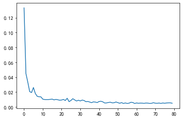

预测
predict = tcn.predict(X_test) real_predict=scaler.inverse_transform(np.concatenate((source_x_test,predict),axis=1)) real_y=scaler.inverse_transform(np.concatenate((source_x_test,Y_test),axis=1)) real_predict=real_predict[:,-1] real_y=real_y[:,-1] 误差评估
plt.figure(figsize=(15,6)) bwith = 0.75 #边框宽度设置为2 ax = plt.gca()#获取边框 ax.spines['bottom'].set_linewidth(bwith) ax.spines['left'].set_linewidth(bwith) ax.spines['top'].set_linewidth(bwith) ax.spines['right'].set_linewidth(bwith) plt.plot(real_predict,label='real_predict') plt.plot(real_y,label='real_y') plt.plot(real_y*(1+0.15),label='15%上限',linestyle='--',color='green') # plt.plot(real_y*(1+0.1),label='10%上限',linestyle='--') # plt.plot(real_y*(1-0.1),label='10%下限',linestyle='--') plt.plot(real_y*(1-0.15),label='15%下限',linestyle='--',color='green') plt.fill_between(range(0,12),real_y*(1+0.15),real_y*(1-0.15),color='gray',alpha=0.2) plt.legend() plt.show() 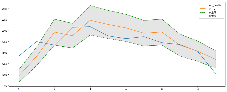
round(mean_squared_error(Y_test,predict),4) 0.0012 from sklearn.metrics import r2_score round(r2_score(real_y,real_predict),4) 0.5192 per_real_loss=(real_y-real_predict)/real_y avg_per_real_loss=sum(abs(per_real_loss))/len(per_real_loss) print(avg_per_real_loss) 0. #计算指定置信水平下的预测准确率 #level为小数 def comput_acc(real,predict,level): num_error=0 for i in range(len(real)): if abs(real[i]-predict[i])/real[i]>level: num_error+=1 return 1-num_error/len(real) comput_acc(real_y,real_predict,0.2),comput_acc(real_y,real_predict,0.15),comput_acc(real_y,real_predict,0.1) (0.75, 0.66667, 0.) 版权声明:本文内容由互联网用户自发贡献,该文观点仅代表作者本人。本站仅提供信息存储空间服务,不拥有所有权,不承担相关法律责任。如发现本站有涉嫌侵权/违法违规的内容, 请联系我们举报,一经查实,本站将立刻删除。
发布者:全栈程序员-站长,转载请注明出处:https://javaforall.net/213828.html原文链接:https://javaforall.net


