强化学习DQN算法

DQN概述

DQN简述

DQN算法主要的算法流程是将神经网络与Q-learning算法结合。利用神经网络强大的表征能力，将高维的输入数据作为强化学习中的state，作为神经网络模型(Agent)的输入; 随后神经网络模型输出每个动作对应的价值(Q值),得到将要执行的动作。强化学习的目标是通过学习从而获得最大的奖励。

接下来将分成神经网络近似价值函数、求解价值网络以及DQN算法效果3个方面简要概述

1. 神经网络近似价值函数

当状态空间和动作空间低维离散时，可以采用基于表格的方法进行求解；当状态空间和动作空间高维连续时，可以基于近似求解法进行求解。值函数近似法通过参数θ使得动作值函数Q(s,a,θ)逼近最优动作值函数Q*(s,a)

 Q(s,a,θ)≈Q*(s,a) 

2. 求解价值网络

3. DQN算法效果

在实践过程中，DQN算法的应用非常广泛，可以根据任务的不同对价值网络及进行针对性的修改，进而完成特定类型的强化学习任务。通过网络的改变，DQN算法可以适应很多应用场景

算法核心

• 目标函数 -基于Q-learning算法构造深度学习可学习函数
• 目标网络 -基于卷积神经网络产生目标Q值，并基于该目标Q值评估下一个状态的Q值
• 经验回访机制 -解决了数据间的相关性和非静态分布的问题

1. 目标函数

θ为卷积神经网络模型的权重参数,其中目标Q值为：

基于当前的Q值和目标Q值的差值可以定义损失函数，得到损失函数之后可以直接使用梯度下降法对卷积神经网络损失函数的权重参数θ进行求解

2. 目标网络

• 预测神经网络
  用来评估当前状态动作对的价值函数；
  
  

• 目标神经网络
  用来目标价值Target Q。
  
  

算法根据损失函数更新预测网络中的参数θ，经过N轮迭代之后，将预测网络的θ复制给目标网络的参数θ-。

3. 经验回放

 (s,a,r,s',T) 

式表示智能体在s状态下执行动作a之后，到达新状态s’,并获得相应地奖励r。其中T为布尔类型，表示新状态s’是否为终止状态

一些案例

• 重力摆案例
• Flappy bird案例

重力摆中地DQN

经验回放

我们将使用经验回放记忆来训练我们的 DQN。它存储智能体观察(observes)到的转换，并允许我们稍后重用这些数据。通过随机采样产生互不相关地小批量数据(batch)。事实证明，这极大地稳定并改进了 DQN 训练过程。

我们需要两个类来实现

• Trainsition – 代表我们环境中单个转换的命名元组。它本质上将（状态，动作）对映射到它们的（next_state，reward）结果，状态是稍后描述的屏幕差异图像。
• RepalyMemory – 一个有界大小的循环缓冲区，用于保存最近观察到的转换。它还实现了.sample() 一种用于选择随机批次转换进行训练的方法。

# 创建一个nametuple对象，拥有属性state,action,next_state,reward Transition = namedtuple('Transition', ('state', 'action', 'next_state', 'reward')) class ReplayMemory(object): def __init__(self, capacity): self.memory = deque([],maxlen=capacity) def push(self, *args): """Save a transition""" self.memory.append(Transition(*args)) def sample(self, batch_size): # random.sample() - 返回从self.memory中随机抽取的batch_size个样本 return random.sample(self.memory, batch_size) def __len__(self): return len(self.memory) 

一个问题：DQN强化学习算法中，最后输出地动作是否要求为简单离散的？

Q网络

class DQN(nn.Module): def __init__(self, h, w, outputs): super(DQN, self).__init__() self.conv1 = nn.Conv2d(3, 16, kernel_size=5, stride=2) self.bn1 = nn.BatchNorm2d(16) self.conv2 = nn.Conv2d(16, 32, kernel_size=5, stride=2) self.bn2 = nn.BatchNorm2d(32) self.conv3 = nn.Conv2d(32, 32, kernel_size=5, stride=2) self.bn3 = nn.BatchNorm2d(32) # Number of Linear input connections depends on output of conv2d layers # and therefore the input image size, so compute it. def conv2d_size_out(size, kernel_size = 5, stride = 2): return (size - (kernel_size - 1) - 1) // stride + 1 convw = conv2d_size_out(conv2d_size_out(conv2d_size_out(w))) convh = conv2d_size_out(conv2d_size_out(conv2d_size_out(h))) linear_input_size = convw * convh * 32 self.head = nn.Linear(linear_input_size, outputs) # Called with either one element to determine next action, or a batch # during optimization. Returns tensor([[left0exp,right0exp]...]). def forward(self, x): x = x.to(device) x = F.relu(self.bn1(self.conv1(x))) x = F.relu(self.bn2(self.conv2(x))) x = F.relu(self.bn3(self.conv3(x))) return self.head(x.view(x.size(0), -1)) 

输入提取

下面的代码是用于从环境中提取和处理渲染图像的实用程序。它使用torchvision包，这使得组合图像转换变得容易。运行该单元后，它将显示它提取的示例补丁。

resize = T.Compose([T.ToPILImage(), T.Resize(40, interpolation=Image.CUBIC), T.ToTensor()]) def get_cart_location(screen_width): world_width = env.x_threshold * 2 scale = screen_width / world_width return int(env.state[0] * scale + screen_width / 2.0) # MIDDLE OF CART def get_screen(): # Returned screen requested by gym is 400x600x3, but is sometimes larger # such as 800x1200x3. Transpose it into torch order (CHW). screen = env.render(mode='rgb_array').transpose((2, 0, 1)) # Cart is in the lower half, so strip off the top and bottom of the screen _, screen_height, screen_width = screen.shape screen = screen[:, int(screen_height*0.4):int(screen_height * 0.8)] view_width = int(screen_width * 0.6) cart_location = get_cart_location(screen_width) if cart_location < view_width // 2: slice_range = slice(view_width) elif cart_location > (screen_width - view_width // 2): slice_range = slice(-view_width, None) else: slice_range = slice(cart_location - view_width // 2, cart_location + view_width // 2) # Strip off the edges, so that we have a square image centered on a cart screen = screen[:, :, slice_range] # Convert to float, rescale, convert to torch tensor # (this doesn't require a copy) screen = np.ascontiguousarray(screen, dtype=np.float32) / 255 screen = torch.from_numpy(screen) # Resize, and add a batch dimension (BCHW) return resize(screen).unsqueeze(0) env.reset() plt.figure() plt.imshow(get_screen().cpu().squeeze(0).permute(1, 2, 0).numpy(), interpolation='none') plt.title('Example extracted screen') plt.show() 

超参数和实用程序

这个单元实例化了我们的模型及其优化器，并定义了一些实用程序：

• select_action– 将根据 epsilon 贪婪策略选择一个动作。简单地说，我们有时会使用我们的模型来选择动作，有时我们只会统一采样。选择随机动作的概率将从 开始，EPS_START 并会以指数方式衰减至EPS_END。EPS_DECAY 控制衰减速度。
• plot_durations– 绘制剧集持续时间的助手，以及过去 100 集的平均值（官方评估中使用的衡量标准）。该图将位于包含主训练循环的单元格下方，并将在每集之后更新。

BATCH_SIZE = 128 GAMMA = 0.999 EPS_START = 0.9 EPS_END = 0.05 EPS_DECAY = 200 TARGET_UPDATE = 10 # Get screen size so that we can initialize layers correctly based on shape # returned from AI gym. Typical dimensions at this point are close to 3x40x90 # which is the result of a clamped and down-scaled render buffer in get_screen() init_screen = get_screen() _, _, screen_height, screen_width = init_screen.shape # Get number of actions from gym action space n_actions = env.action_space.n policy_net = DQN(screen_height, screen_width, n_actions).to(device) target_net = DQN(screen_height, screen_width, n_actions).to(device) target_net.load_state_dict(policy_net.state_dict()) target_net.eval() optimizer = optim.RMSprop(policy_net.parameters()) memory = ReplayMemory(10000) steps_done = 0 def select_action(state): global steps_done sample = random.random() eps_threshold = EPS_END + (EPS_START - EPS_END) * \ math.exp(-1. * steps_done / EPS_DECAY) steps_done += 1 if sample > eps_threshold: with torch.no_grad(): # t.max(1) will return largest column value of each row. # second column on max result is index of where max element was # found, so we pick action with the larger expected reward. return policy_net(state).max(1)[1].view(1, 1) else: return torch.tensor([[random.randrange(n_actions)]], device=device, dtype=torch.long) episode_durations = [] def plot_durations(): plt.figure(2) plt.clf() durations_t = torch.tensor(episode_durations, dtype=torch.float) plt.title('Training...') plt.xlabel('Episode') plt.ylabel('Duration') plt.plot(durations_t.numpy()) # Take 100 episode averages and plot them too if len(durations_t) >= 100: means = durations_t.unfold(0, 100, 1).mean(1).view(-1) means = torch.cat((torch.zeros(99), means)) plt.plot(means.numpy()) plt.pause(0.001) # pause a bit so that plots are updated if is_ipython: display.clear_output(wait=True) display.display(plt.gcf()) 

训练循环

最后是训练我们模型的代码。

def optimize_model(): if len(memory) < BATCH_SIZE: return transitions = memory.sample(BATCH_SIZE) # Transpose the batch (see https://stackoverflow.com/a/19343/ for # detailed explanation). This converts batch-array of Transitions # to Transition of batch-arrays. batch = Transition(*zip(*transitions)) # Compute a mask of non-final states and concatenate the batch elements # (a final state would've been the one after which simulation ended) non_final_mask = torch.tensor(tuple(map(lambda s: s is not None, batch.next_state)), device=device, dtype=torch.bool) non_final_next_states = torch.cat([s for s in batch.next_state if s is not None]) state_batch = torch.cat(batch.state) action_batch = torch.cat(batch.action) reward_batch = torch.cat(batch.reward) # Compute Q(s_t, a) - the model computes Q(s_t), then we select the # columns of actions taken. These are the actions which would've been taken # for each batch state according to policy_net state_action_values = policy_net(state_batch).gather(1, action_batch) # Compute V(s_{t+1}) for all next states. # Expected values of actions for non_final_next_states are computed based # on the "older" target_net; selecting their best reward with max(1)[0]. # This is merged based on the mask, such that we'll have either the expected # state value or 0 in case the state was final. next_state_values = torch.zeros(BATCH_SIZE, device=device) next_state_values[non_final_mask] = target_net(non_final_next_states).max(1)[0].detach() # Compute the expected Q values expected_state_action_values = (next_state_values * GAMMA) + reward_batch # Compute Huber loss criterion = nn.SmoothL1Loss() loss = criterion(state_action_values, expected_state_action_values.unsqueeze(1)) # Optimize the model optimizer.zero_grad() loss.backward() for param in policy_net.parameters(): param.grad.data.clamp_(-1, 1) optimizer.step() 

在下面，您可以找到主要的训练循环。一开始我们重置环境并初始化state张量。然后，我们采样一个动作，执行它，观察下一个屏幕和奖励（总是 1），并优化我们的模型一次。当情节结束时（我们的模型失败），我们重新开始循环。

下面，num_episodes设置的很小。您应该下载笔记本并运行更多的 episoode，例如 300+ 以获得有意义的持续时间改进。

num_episodes = 50 for i_episode in range(num_episodes): # Initialize the environment and state env.reset() last_screen = get_screen() current_screen = get_screen() state = current_screen - last_screen for t in count(): # Select and perform an action action = select_action(state) _, reward, done, _ = env.step(action.item()) reward = torch.tensor([reward], device=device) # Observe new state last_screen = current_screen current_screen = get_screen() if not done: next_state = current_screen - last_screen else: next_state = None # Store the transition in memory memory.push(state, action, next_state, reward) # Move to the next state state = next_state # Perform one step of the optimization (on the policy network) optimize_model() if done: episode_durations.append(t + 1) plot_durations() break # Update the target network, copying all weights and biases in DQN if i_episode % TARGET_UPDATE == 0: target_net.load_state_dict(policy_net.state_dict()) print('Complete') env.render() env.close() plt.ioff() plt.show() 

下面的图说明了整个结果数据流。

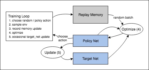
动作是随机选择的或基于策略选择的，从健身房环境中获取下一步样本。我们将结果记录在回放内存中，并在每次迭代中运行优化步骤。优化从重放内存中随机选择一批来训练新策略。“旧的” target_net 也用于优化以计算预期Q值；它不时更新以保持最新状态。