【深度学习】 基于Keras的Attention机制代码实现及剖析——Dense+Attention

说明

1. 大部分代码来源于网上，但网上的代码一下子可能难以入门或因版本原因报错，此处整理后进行详细分析。
     参考的代码来源1：Attention mechanism Implementation for Keras.网上大部分代码都源于此，直接使用时注意Keras版本，若版本不对应，在merge处会报错，解决办法为：导入Multiply层并将attention_dense.py第17行的：
   attention_mul = merge([inputs, attention_probs], output_shape=32, name=‘attention_mul’, mode=‘mul’)，改为：attention_mul = Multiply()([inputs, attention_probs])即可。
     参考的代码来源2：[深度应用]·Keras极简实现Attention结构。这相当于来源1的简化版本，其将注意力层还做了封装，可直接使用。但此方法运用了两个注意力层，使我有些不太理解，这个问题在后面会进行讨论。
     本文主体将在来源1的基础上进行分析探讨。

   
   
   
   
   
   
   
   

2. Attention机制大致过程就是分配权重，所有用到权重的地方都可以考虑使用它，另外它是一种思路，不局限于深度学习的实现方法，此处仅代码上分析，且为深度学习的实现版本。更多理论请看解读大牛文章深度学习中的注意力机制(2017版)，还可以看解读这篇文章的大牛文章：[深度概念]·Attention机制实践解读。
3. 此处仅介绍Dense+Attention，进阶篇LSTM+Attention请看【深度学习】 基于Keras的Attention机制代码实现及剖析——LSTM+Attention。

实验目的

1. 在简单的分类模型(如最简的全连接网络)基础上实现Attention机制的运用。
2. 检验Attention是否真的捕捉到了关键特征，即被Attention分配的关键特征的权重是否更高。
3. 在已有的模型基础上适当做些变化，如调参或新加层，看看Attention的稳定性如何。

数据集构造

def get_data(n, input_dim, attention_column=1): """ Data generation. x is purely random except that it's first value equals the target y. In practice, the network should learn that the target = x[attention_column]. Therefore, most of its attention should be focused on the value addressed by attention_column. :param n: the number of samples to retrieve. :param input_dim: the number of dimensions of each element in the series. :param attention_column: the column linked to the target. Everything else is purely random. :return: x: model inputs, y: model targets """ x = np.random.standard_normal(size=(n, input_dim)) y = np.random.randint(low=0, high=2, size=(n, 1)) x[:, attention_column] = y[:, 0] return x, y 

模型搭建

  下面开始在单隐层全连接网络的基础上用keras搭建注意力层。

def build_model(): K.clear_session() #清除之前的模型，省得压满内存 inputs = Input(shape=(input_dim,)) #输入层 # ATTENTION PART STARTS HERE 注意力层 attention_probs = Dense(input_dim, activation='softmax', name='attention_vec')(inputs) attention_mul = Multiply()([inputs, attention_probs]) # ATTENTION PART FINISHES HERE attention_mul = Dense(64)(attention_mul) #原始的全连接 output = Dense(1, activation='sigmoid')(attention_mul) #输出层 model = Model(input=[inputs], output=output) return model 

模型训练及验证

  设置随机种子可以调试对比每次结果的异同，输入必要参数，调用模型就可以开始训练了，由于是二分类问题，所以损失函数用二分类交叉熵。训练集测试集8:2进行验证。

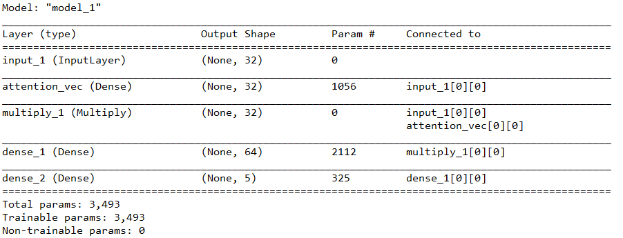
if __name__ == '__main__': np.random.seed(1337) # for reproducibility input_dim = 32 #特征数 N = 10000 #数据集总记录数 inputs_1, outputs = get_data(N, input_dim) #构造数据集 m = build_model() #构造模型 m.compile(optimizer='adam', loss='binary_crossentropy', metrics=['accuracy']) m.summary() m.fit([inputs_1], outputs, epochs=20, batch_size=64, validation_split=0.2) 

def get_activations(model, inputs, print_shape_only=False, layer_name=None): # Documentation is available online on Github at the address below. # From: https://github.com/philipperemy/keras-visualize-activations print('----- activations -----') activations = [] inp = model.input if layer_name is None: outputs = [layer.output for layer in model.layers] else: outputs = [layer.output for layer in model.layers if layer.name == layer_name] # all layer outputs funcs = [K.function([inp] + [K.learning_phase()], [out]) for out in outputs] # evaluation functions layer_outputs = [func([inputs, 1.])[0] for func in funcs] for layer_activations in layer_outputs: activations.append(layer_activations) if print_shape_only: print(layer_activations.shape) else: print(layer_activations) return activations 

  这个函数有些复杂，但只需要知道它的功能就行，下面我们在main函数里续写如下代码进行调用：

 testing_inputs_1, testing_outputs = get_data(1, input_dim) # Attention vector corresponds to the second matrix. # The first one is the Inputs output. attention_vector = get_activations(m, testing_inputs_1, print_shape_only=True, layer_name='attention_vec')[0].flatten() print('attention =', attention_vector) # plot part. pd.DataFrame(attention_vector, columns=['attention (%)']).plot(kind='bar', title='Attention Mechanism as ' 'a function of input' ' dimensions.') plt.show() 

from keras.models import * from keras.layers import Input, Dense, Multiply import keras.backend as K import numpy as np import matplotlib.pyplot as plt import pandas as pd def get_activations(model, inputs, print_shape_only=False, layer_name=None): # Documentation is available online on Github at the address below. # From: https://github.com/philipperemy/keras-visualize-activations print('----- activations -----') activations = [] inp = model.input if layer_name is None: outputs = [layer.output for layer in model.layers] else: outputs = [layer.output for layer in model.layers if layer.name == layer_name] # all layer outputs funcs = [K.function([inp] + [K.learning_phase()], [out]) for out in outputs] # evaluation functions layer_outputs = [func([inputs, 1.])[0] for func in funcs] for layer_activations in layer_outputs: activations.append(layer_activations) if print_shape_only: print(layer_activations.shape) else: print(layer_activations) return activations def get_data(n, input_dim, attention_column=1): """ Data generation. x is purely random except that it's first value equals the target y. In practice, the network should learn that the target = x[attention_column]. Therefore, most of its attention should be focused on the value addressed by attention_column. :param n: the number of samples to retrieve. :param input_dim: the number of dimensions of each element in the series. :param attention_column: the column linked to the target. Everything else is purely random. :return: x: model inputs, y: model targets """ x = np.random.standard_normal(size=(n, input_dim)) y = np.random.randint(low=0, high=2, size=(n, 1)) x[:, attention_column] = y[:, 0] return x, y def build_model(): K.clear_session() #清除之前的模型，省得压满内存 inputs = Input(shape=(input_dim,)) #输入层 # ATTENTION PART STARTS HERE 注意力层 attention_probs = Dense(input_dim, activation='softmax', name='attention_vec')(inputs) attention_mul = Multiply()([inputs, attention_probs]) # ATTENTION PART FINISHES HERE attention_mul = Dense(64)(attention_mul) #原始的全连接 output = Dense(1, activation='sigmoid')(attention_mul) #输出层 model = Model(inputs=[inputs], outputs=output) return model if __name__ == '__main__': np.random.seed(1337) # for reproducibility input_dim = 32 #特征数 N = 10000 #数据集总记录数 inputs_1, outputs = get_data(N, input_dim) #构造数据集 m = build_model() #构造模型 m.compile(optimizer='adam', loss='binary_crossentropy', metrics=['accuracy']) m.summary() m.fit([inputs_1], outputs, epochs=20, batch_size=64, validation_split=0.2) testing_inputs_1, testing_outputs = get_data(1, input_dim) # Attention vector corresponds to the second matrix. # The first one is the Inputs output. attention_vector = get_activations(m, testing_inputs_1, print_shape_only=True, layer_name='attention_vec')[0].flatten() print('attention =', attention_vector) # plot part. pd.DataFrame(attention_vector, columns=['attention (%)']).plot(kind='bar', title='Attention Mechanism as ' 'a function of input' ' dimensions.') plt.show() 

拓展

  以上是对别人的代码的学习理解，接下来做一些小改动，看看Attention表现如何。

多分类问题时，Attention效果如何？

  以上代码改为多分类，需要注意一下几点：

1. 构造数据集时，randint的high置为类别个数。
2. 将随机完毕的y由十进制数改为二进制one-hot形式，以待模型输入。
3. 模型最后一层的结点个数置为类别个数，同时激活函数改为softmax。
4. 损失函数改为：loss=‘categorical_crossentropy’

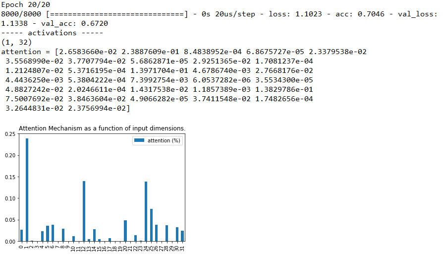
  我们将类别数设置为5，先看看结果：

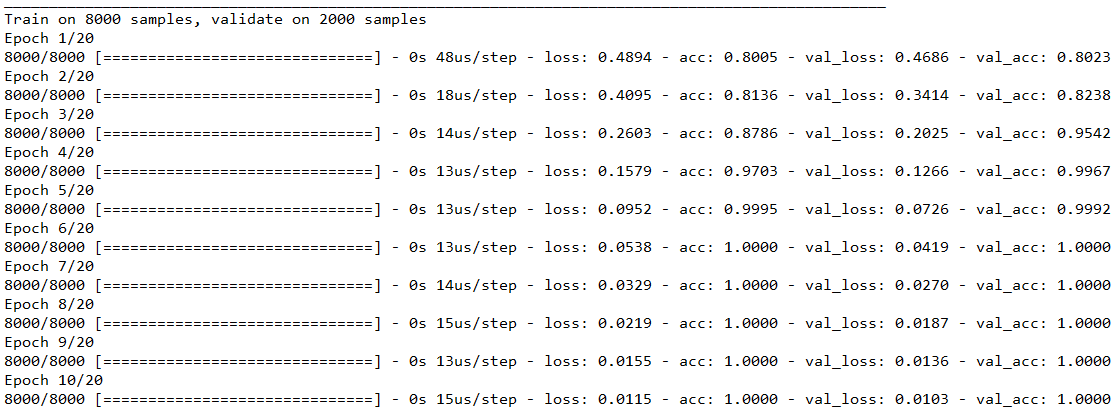
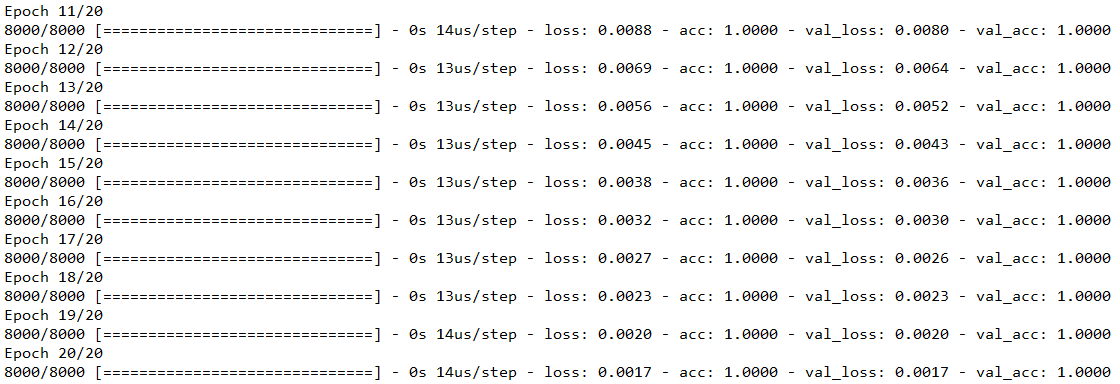
  可以看到还是很轻松就学出了规律，再看看可视化的权重：

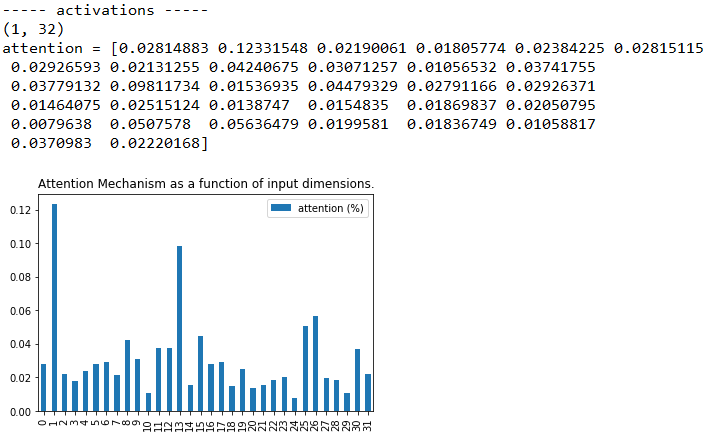
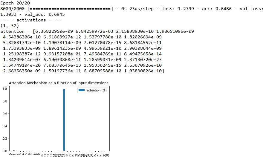
  对比可以发现，尽管“第1列”的权重仍是最高的，但这个优势已经不明显了，注意力机制的健壮性如何？是否因为是多分类，效果就下降了呢？那么增大类别个数来看看，我们将类别个数置为20，直接看图：

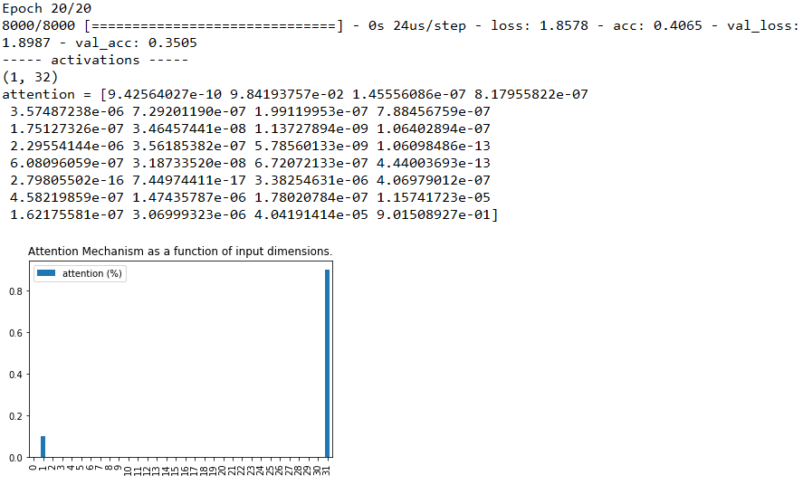
  可以观察到，“第1列”仍是最高的权重，并且比5分类时还要高，说明注意力机制确实非常强大，可我还是不死心，那么继续调，30个类的时候如何呢？

  综合这两张图，我们惊奇地发现，准确率下降了，注意力紊乱了！注意力没有集中在本来人工设置最特别的特征“第1列”上，而集中出现在“第17列”上，这是为什么呢？继续尝试看看，设为50，100，图片分别为：


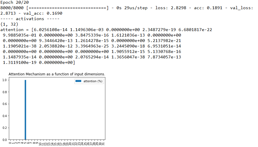
  可以发现，“注意力紊乱” 的情况仍存在，即使注意力没有向我们预设的“焦点”集中，分类准确率降低到了16.9% 这种“注意力紊乱”的表现是因为什么呢？
  我们可以发现，原模型设置的特征数是32个，当分类数接近或者超过特征数时，注意力才发生紊乱，而特征数对应的就是权重数，也就是注意力层的“算力”。因此我们可以有如下猜测：注意力紊乱是因为问题规模变大，导致原先的学习能力不足，学的不好。
  对于做DL的人来讲，很容易能想到，学得不够好怎么办？加层里的结点数量！加网络的深度！我们将分类数设置为50，特征数设置为128看看效果：


  果然，注意力又能“集中”了，但分类效果依旧很差。那么再试试加深，我们将注意力里的全连接层，多增加一层，分类数设置为50，特征数设置为32，再看看效果：

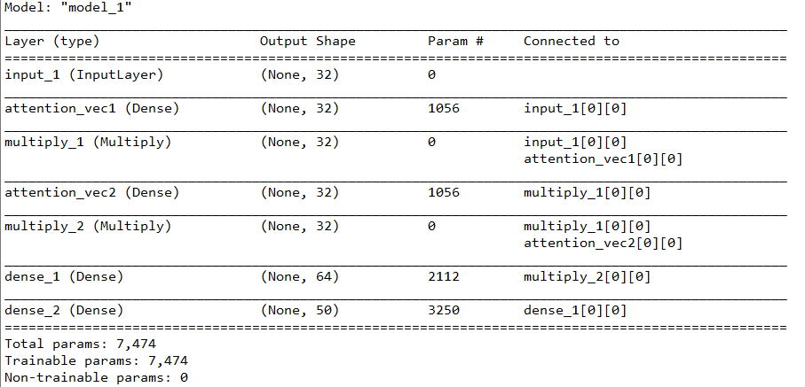
  加深注意力网络后不仅注意力回归了，准确率也上升了！(重大发现啊！那是不是可以发文章了呢？)，然鹅已经有大佬在2016年就已经发表了，还给了一个好听的名字：多层注意力网络(Hierarchical Attention Networks)，论文名字是Hierarchical Attention Networks for Document Classification。还有谷歌大佬也提出了一个方法来增加算力，叫多头注意力机制(multi-headed self-attention)，论文名字为：Attention Is All You Need。

拓展总结

  在拓展中，我们可以发现，注意力机制的效果在算力充足的情况下，是能很好捕捉重点特征的，而针对注意力算力的不足，可以使用加结点和加层级的方法，但加结点会增加特征，这与现实中客观任务不符(即分类的数据集特征一般是固定的)，且准确率没有提升，而加层级已有人进行应用并证实有效，因此可以作为我们搭建自己网络，提高自己指标的一个小技巧。
  此次扩展的完整代码(仅到多分类)：

from keras.models import * from keras.layers import Input, Dense, Multiply import keras.backend as K import numpy as np import matplotlib.pyplot as plt import pandas as pd from keras.utils import to_categorical def get_activations(model, inputs, print_shape_only=False, layer_name=None): # Documentation is available online on Github at the address below. # From: https://github.com/philipperemy/keras-visualize-activations print('----- activations -----') activations = [] inp = model.input if layer_name is None: outputs = [layer.output for layer in model.layers] else: outputs = [layer.output for layer in model.layers if layer.name == layer_name] # all layer outputs funcs = [K.function([inp] + [K.learning_phase()], [out]) for out in outputs] # evaluation functions layer_outputs = [func([inputs, 1.])[0] for func in funcs] for layer_activations in layer_outputs: activations.append(layer_activations) if print_shape_only: print(layer_activations.shape) else: print(layer_activations) return activations def get_data(n, input_dim, class_num, attention_column=1): """ Data generation. x is purely random except that it's first value equals the target y. In practice, the network should learn that the target = x[attention_column]. Therefore, most of its attention should be focused on the value addressed by attention_column. :param n: the number of samples to retrieve. :param input_dim: the number of dimensions of each element in the series. :param attention_column: the column linked to the target. Everything else is purely random. :return: x: model inputs, y: model targets """ x = np.random.standard_normal(size=(n, input_dim)) y = np.random.randint(low=0, high=class_num, size=(n, 1)) x[:, attention_column] = y[:, 0] y = np.array([to_categorical(yy,class_num) for yy in y]).reshape(n,class_num) return x, y def build_model(input_dim,class_num): K.clear_session() #清除之前的模型，省得压满内存 inputs = Input(shape=(input_dim,)) #输入层 # ATTENTION PART STARTS HERE 注意力层 attention_probs = Dense(input_dim, activation='softmax', name='attention_vec')(inputs) attention_mul = Multiply()([inputs, attention_probs]) # ATTENTION PART FINISHES HERE attention_mul = Dense(64)(attention_mul) #原始的全连接 output = Dense(class_num, activation='softmax')(attention_mul) #输出层 model = Model(inputs=[inputs], outputs=output) return model if __name__ == '__main__': np.random.seed(1337) # for reproducibility input_dim = 32 #特征数 N = 10000 #数据集总记录数 class_num = 20 #类别数 inputs_1, outputs = get_data(N, input_dim, class_num) #构造数据集 m = build_model(input_dim,class_num) #构造模型 m.compile(optimizer='adam', loss='categorical_crossentropy', metrics=['accuracy']) m.summary() m.fit([inputs_1], outputs, epochs=20, batch_size=64, validation_split=0.2) testing_inputs_1, testing_outputs = get_data(1, input_dim, class_num) # Attention vector corresponds to the second matrix. # The first one is the Inputs output. attention_vector = get_activations(m, testing_inputs_1, print_shape_only=True, layer_name='attention_vec')[0].flatten() print('attention =', attention_vector) # plot part. pd.DataFrame(attention_vector, columns=['attention (%)']).plot(kind='bar', title='Attention Mechanism as ' 'a function of input' ' dimensions.') plt.show()