PINN学习记录（2）

PINN学习记录（2）

PINN基于解物理的方程的应用，所以我自己学习了一段时间，参考了网上很多的开源项目，末尾会贴出一些，自己总结了一下思路

解微分方程

1、ODE

$f^{\prime }(x)=f(x)$
$f(0)=1$

网络构造

这里说明一下，之后用nn.module，来解决，这只是建立一个通用网络

import torch import torch.nn as nn import numpy as np class Net(nn.Module): def __init__(self, NL, NN): # NL是有多少层隐藏层 # NN是每层的神经元数量 super(Net, self).__init__() self.input_layer = nn.Linear(1, NN) self.hidden_layer = nn.ModuleList([nn.Linear(NN, NN) for i in range(NL)]) self.output_layer = nn.Linear(NN, 1) def forward(self, x): o = self.act(self.input_layer(x)) for i, li in enumerate(self.hidden_layer): o = self.act(li(o)) out = self.output_layer(o) return out def act(self, x): return torch.tanh(x) 

网络，损失，优化声明

net=Net(4,20) mse_cost_function = torch.nn.MSELoss(reduction='mean') # Mean squared error optimizer = torch.optim.Adam(net.parameters(),lr=1e-4) 

ode建立

def ode_01(x,net): y=net(x) y_x = torch.autograd.grad(y, x,grad_outputs=torch.ones_like(net(x)),create_graph=True)[0] return y-y_x 

注意：对于torch.autograd.grad，如果没有说明grad_outputs,就用y.sum()

训练

iterations=1000 for epoch in range(iterations): # Loss based on initial value x_in = np.random.uniform(low=0.0, high=2.0, size=(2000, 1)) pt_x_in = Variable(torch.from_numpy(x_in).float(), requires_grad=True) y = torch.exp(pt_x_in)#与真实值作比较 y_0 = net(torch.zeros( 2000,1)) mse_i = mse_cost_function(y_0, torch.ones( 2000,1)) optimizer.zero_grad() # to make the gradients zero # Loss based on ODE pt_all_zeros= Variable(torch.from_numpy(np.zeros((2000,1))).float(), requires_grad=False) pt_y_colection=ode_01(pt_x_in,net) mse_f=mse_cost_function(pt_y_colection,pt_all_zeros) # Combining the loss functions loss = mse_i+ mse_f #y_train测试 y_train0 = net(pt_x_in) loss.backward() # This is for computing gradients using backward propagation optimizer.step() # This is equivalent to : theta_new = theta_old - alpha * derivative of J w.r.t theta if epoch%1000==0: print(epoch, "Traning Loss:", loss.data) print(f'times { 
     epoch} - loss: { 
     loss.item()} - y_0: { 
     y_0}') plt.cla() plt.scatter(pt_x_in.detach().numpy(), y.detach().numpy()) plt.scatter(pt_x_in.detach().numpy(), y_train0.detach().numpy(),c='red') plt.pause(0.1) 

完整CODE

from mylayer import Net import torch import torch.nn as nn import numpy as np import matplotlib.pyplot as plt import torch.optim as optim from torch.autograd import Variable """ NOTE:当用linspace生成，作图可以用plot 但换成uniform，必须用scatter 否则图形会因为随机取样而失真 """ class MyNet(torch.nn.Module): def __init__(self): super(MyNet, self).__init__() # 第一句话，调用父类的构造函数 self.mylayer1 = Net() def forward(self, a): x = self.mylayer1(a) return x """ 用神经网络模拟微分方程,f(x)'=f(x),初始条件f(0) = 1 """ net=Net(4,20) mse_cost_function = torch.nn.MSELoss(reduction='mean') # Mean squared error optimizer = torch.optim.Adam(net.parameters(),lr=1e-4) def ode_01(x,net): y=net(x) y_x = torch.autograd.grad(y, x,grad_outputs=torch.ones_like(net(x)),create_graph=True)[0] return y-y_x iterations=104 #可以试试用linspace也可以做出来 #x_i = torch.linspace(0, 2, 2000, requires_grad=True).unsqueeze(-1) plt.ion() for epoch in range(iterations): # Loss based on initial value x_bc = np.zeros((500, 1)) x_in = np.random.uniform(low=0.0, high=2.0, size=(2000, 1)) pt_x_in = Variable(torch.from_numpy(x_in).float(), requires_grad=True) y = torch.exp(pt_x_in) y_0 = net(torch.zeros( 2000,1)) y_train0 = net(pt_x_in) mse_i = mse_cost_function(y_0, torch.ones( 2000,1)) optimizer.zero_grad() # to make the gradients zero # Loss based on PDE pt_all_zeros= Variable(torch.from_numpy(np.zeros((2000,1))).float(), requires_grad=False) pt_y_colection=ode_01(pt_x_in,net) mse_f=mse_cost_function(pt_y_colection,pt_all_zeros) # Combining the loss functions loss = mse_i+ mse_f loss.backward() # This is for computing gradients using backward propagation optimizer.step() # This is equivalent to : theta_new = theta_old - alpha * derivative of J w.r.t theta if epoch%1000==0: print(epoch, "Traning Loss:", loss.data) print(f'times { 
     epoch} - loss: { 
     loss.item()} - y_0: { 
     y_0}') plt.cla() plt.scatter(pt_x_in.detach().numpy(), y.detach().numpy()) plt.scatter(pt_x_in.detach().numpy(), y_train0.detach().numpy(),c='red') plt.pause(0.1) 

2、PDE

网络构造

import torch import torch.nn as nn import numpy as np class Net(nn.Module): def __init__(self, NL, NN): # NL是有多少层隐藏层 # NN是每层的神经元数量 super(Net, self).__init__() self.input_layer = nn.Linear(2, NN) self.hidden_layer = nn.ModuleList([nn.Linear(NN, NN) for i in range(NL)]) self.output_layer = nn.Linear(NN, 1) def forward(self, x): o = self.act(self.input_layer(x)) for i, li in enumerate(self.hidden_layer): o = self.act(li(o)) out = self.output_layer(o) return out def act(self, x): return torch.tanh(x) 

输入改2即可

网络，损失，优化声明

net=Net(4,30) mse_cost_function = torch.nn.MSELoss(reduction='mean') # Mean squared error optimizer = torch.optim.Adam(net.parameters(),lr=1e-4) 

pde

def f(x): u = net(x) u_x = torch.autograd.grad(u, x,grad_outputs=torch.ones_like(net(x)), create_graph=True,allow_unused=True) u_t = torch.autograd.grad(u, x,grad_outputs=torch.ones_like(net(x)), create_graph=True,allow_unused=True) d_x= u_x[0][:, 1].unsqueeze(-1) d_t = u_t[0][:, 0].unsqueeze(-1) u_xx=torch.autograd.grad(d_x, x, grad_outputs=torch.ones_like(d_x), create_graph=True,allow_unused=True)[0][:, 1].unsqueeze(-1) w = torch.tensor(0.01 / np.pi) f = d_t + u * d_x - w * u_xx return f 

这里卡了一下，因为我一开始u_x = torch.autograd.grad(u, x[:,1],grad_outputs=torch.ones_like(net(x)), create_graph=True,allow_unused=True)
这样会报错

边界和初始值

#boundary t_bc = np.zeros((2000,1)) x_bc = np.random.uniform(low=-1.0, high=1.0, size=(2000,1)) # compute u based on BC u_bc = -np.sin(np.pi*x_bc) #initial x_inr=np.ones((2000,1)) x_inl=-np.ones((2000,1)) t_in=np.random.uniform(low=0, high=1.0, size=(2000,1)) u_in= np.zeros((2000,1)) 

训练

for epoch in range(iterations): optimizer.zero_grad() # to make the gradients zero # Loss based on boundary conditions pt_x_bc = Variable(torch.from_numpy(x_bc).float(), requires_grad=False) pt_t_bc = Variable(torch.from_numpy(t_bc).float(), requires_grad=False) pt_u_bc = Variable(torch.from_numpy(u_bc).float(), requires_grad=False) net_bc_out = net(torch.cat([ pt_t_bc,pt_x_bc],1)) # output of u(x,t) mse_u1 = mse_cost_function(net_bc_out, pt_u_bc) # Loss based on initial value pt_x_inr = Variable(torch.from_numpy(x_inr).float(), requires_grad=False) pt_x_inl = Variable(torch.from_numpy(x_inl).float(), requires_grad=False) pt_t_in = Variable(torch.from_numpy(t_in).float(), requires_grad=False) pt_u_in = Variable(torch.from_numpy(u_in).float(), requires_grad=False) net_bc_inr = net(torch.cat([ pt_t_in,pt_x_inr],1)) # output of u(x,t) net_bc_inl = net(torch.cat([ pt_t_in,pt_x_inl],1)) mse_u2r = mse_cost_function(net_bc_inr, pt_u_in) mse_u2l = mse_cost_function(net_bc_inl, pt_u_in) # Loss based on PDE x_collocation = np.random.uniform(low=-1.0, high=1.0, size=(2000, 1)) t_collocation = np.random.uniform(low=0.0, high=1.0, size=(2000, 1)) all_zeros = np.zeros((2000, 1)) pt_x_collocation = Variable(torch.from_numpy(x_collocation).float(), requires_grad=True) pt_t_collocation = Variable(torch.from_numpy(t_collocation).float(), requires_grad=True) pt_all_zeros = Variable(torch.from_numpy(all_zeros).float(), requires_grad=False) f_out = f(torch.cat([pt_t_collocation, pt_x_collocation],1)) # output of f(x,t) mse_f = mse_cost_function(f_out, pt_all_zeros) # Combining the loss functions loss = mse_u1+mse_u2r+mse_u2l + mse_f loss.backward() # This is for computing gradients using backward propagation optimizer.step() # This is equivalent to : theta_new = theta_old - alpha * derivative of J w.r.t theta with torch.autograd.no_grad(): if epoch%1000==0: print(epoch, "Traning Loss:", loss.data) 

画图

#画图 from matplotlib import cm t = np.linspace(0,1,100) x = np.linspace(-1,1,256) ms_t, ms_x = np.meshgrid(t, x) x = np.ravel(ms_x).reshape(-1, 1) t = np.ravel(ms_t).reshape(-1, 1) pt_x = Variable(torch.from_numpy(x).float(), requires_grad=True) pt_t = Variable(torch.from_numpy(t).float(), requires_grad=True) pt_u0 = net(torch.cat([pt_t,pt_x],1)) u = pt_u0.data.cpu().numpy() pt_u0=u.reshape(256,100) fig = plt.figure() ax = fig.add_subplot(projection='3d') ax.set_zlim([-1, 1]) ax.plot_surface(ms_t, ms_x, pt_u0, cmap=cm.RdYlBu_r, edgecolor='blue', linewidth=0.0003, antialiased=True) ax.set_xlabel('t') ax.set_ylabel('x') ax.set_zlabel('u') plt.savefig('Preddata.png') plt.close(fig) 

fig = plt.figure() ax = fig.gca(projection='3d') x = np.arange(-1, 1, 0.02) t = np.arange(0, 1, 0.02) ms_x, ms_t = np.meshgrid(x, t) # Just because meshgrid is used, we need to do the following adjustment x = np.ravel(ms_x).reshape(-1, 1) t = np.ravel(ms_t).reshape(-1, 1) pt_x = Variable(torch.from_numpy(x).float(), requires_grad=True).to(device) pt_t = Variable(torch.from_numpy(t).float(), requires_grad=True).to(device) pt_u = net(pt_x, pt_t) u = pt_u.data.cpu().numpy() ms_u = u.reshape(ms_t.shape) surf = ax.plot_surface(ms_x, ms_t, ms_u, cmap=cm.coolwarm, linewidth=0, antialiased=False) ax.zaxis.set_major_locator(LinearLocator(10)) ax.zaxis.set_major_formatter(FormatStrFormatter('%.02f')) fig.colorbar(surf, shrink=0.5, aspect=5) plt.show() 

结果

1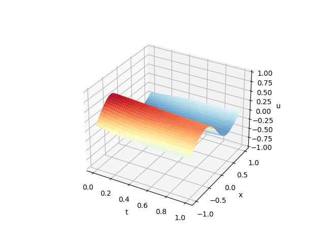

2