
大家好,又见面了,我是你们的朋友全栈君。如果您正在找激活码,请点击查看最新教程,关注关注公众号 “全栈程序员社区” 获取激活教程,可能之前旧版本教程已经失效.最新Idea2022.1教程亲测有效,一键激活。
Jetbrains全系列IDE稳定放心使用
文章目录
STN的作用
之前参加过一个点云数据分类的比赛,主要借鉴了PointNet的网络结构,在PointNet中使用到了两次STN。点云数据存在两个主要问题:1、无序性:点云本质上是一长串点(nx3矩阵,其中n是点数)。在几何上,点的顺序不影响它在空间中对整体形状的表示,例如,相同的点云可以由两个完全不同的矩阵表示。2、旋转性:相同的点云在空间中经过一定的刚性变化(旋转或平移),坐标发生变化,我们希望不论点云在怎样的坐标系下呈现,网络都能正确的识别出。
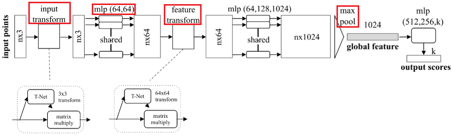

上图是PointNet的网络结构,网络对每个点进行了一定程度的特征提取之后,maxpooling可以对点云的整体提取出global feature,从而解决了无序性的问题。PointNet采用了两次STN解决旋转行问题,第一次input transform是对空间中点云进行调整,直观上理解是旋转出一个更有利于分类或分割的角度,比如把物体转到正面;第二次feature transform是对提取出的64维特征进行对齐,即在特征层面对点云进行变换。PointNet是第一篇直接使用原始点云数据作为输入进行分类和分割任务的论文,有兴趣的可以看一下原文PointNet: Deep Learning on Point Sets for 3D Classification and Segmentation
PointNet中的STN实现了三位点云的旋转,而最初出自这篇Spatial Transformer Networks论文的STN是针对图片提出的,但其目的是一致的,都是为了实现旋转不变性。
熟悉卷积网络和池化过程的人应该知道,普通的CNN能够显式的学习平移不变性,以及隐式的学习旋转不变性,那为什么还需要STN? Attention机制告诉了我们,与其让网络隐式的学习到某种能力,不如为网络设计一个显式的处理模块,专门处理所需的各种变换。STN把裁剪、平移、缩放等过程加入了训练,使其可以求解梯度,参与网络的反向传播,有利于End-to-end网络的设计与实现。
STN的基本结构
STN的核心结构如下图所示:
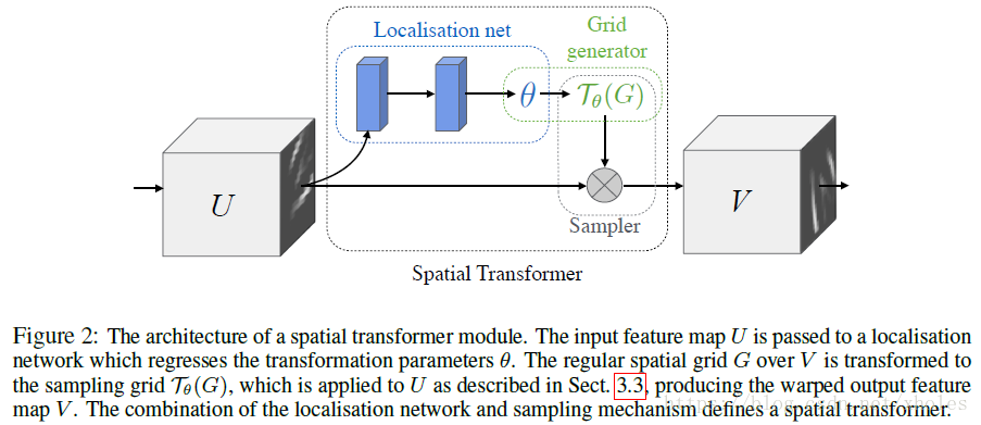
主要由三个部分组成:1、参数预测:Localisation net ;2、坐标映射:Grid generator ;3、像素的采集:Sampler
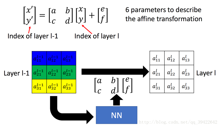
关于平移、缩放和旋转的具体转换原理,这篇博客里有更详细的介绍,这里只需要知道通过六个参数就可以实现这些操作即可,因此STN的输出也就是一个2×3的转换矩阵,转换公式如下:
而在论文中公式写作:
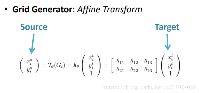
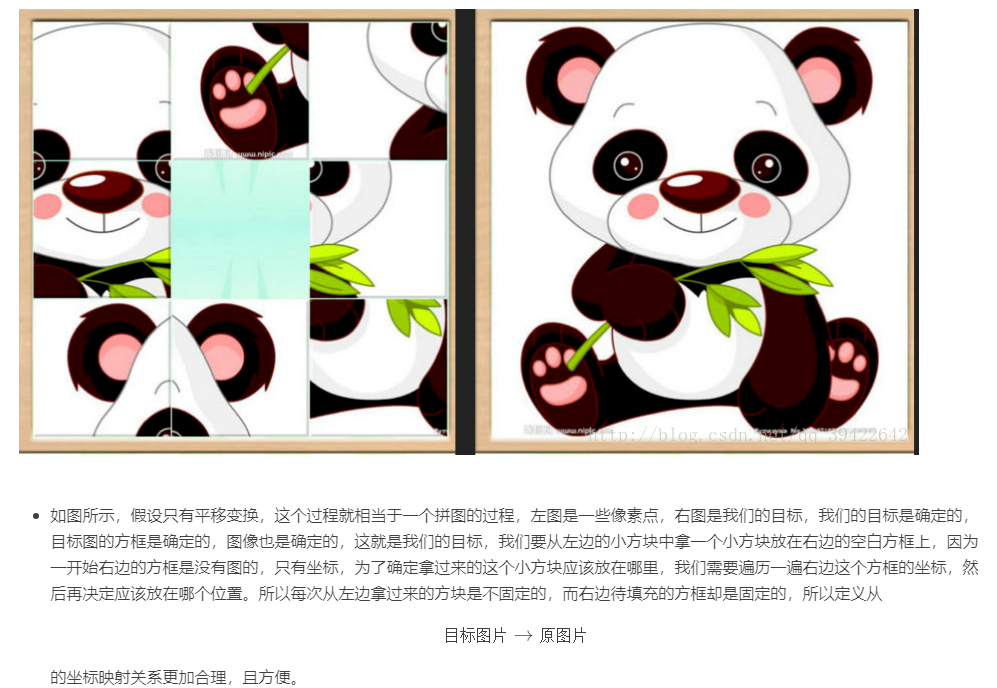
需要注意的是,(xti,yti)是输出的目标图片的坐标,(xsi,ysi)是原图片的坐标,Aθ表示仿射关系即STN矩阵,也就是说转换矩阵是目标图片到原图片的映射。比较合理的解释是:坐标映射的作用是让目标图片在原图片上采样,每次从原图片上不同坐标采集像素到目标图片上,原图片上会有多余的信息,而目标图片最终一定会被填满。每次目标图片的坐标要遍历一遍,是固定的,而采集原图的坐标是不固定的。通过拼图的例子会更容易理解:
在了解坐标变换原理后,先简单概括一下三个模块的主要工作:
1、Localisation net:在输入特征映射上应用卷积或FC层,获取到2×3的仿射变换矩阵参数θ
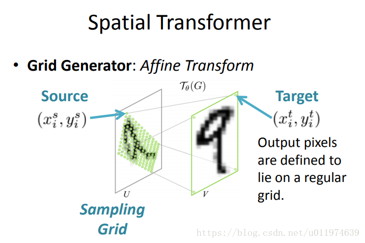
2、Grid generator:输出采样网格,即目标图片V中的第(i,j)个位置,对应于原图片U中的哪一个位置。在仿射变换下,可以理解为如下图的过程,通过目标采样网格经过仿射变换获取到实际在输入上采样网格点
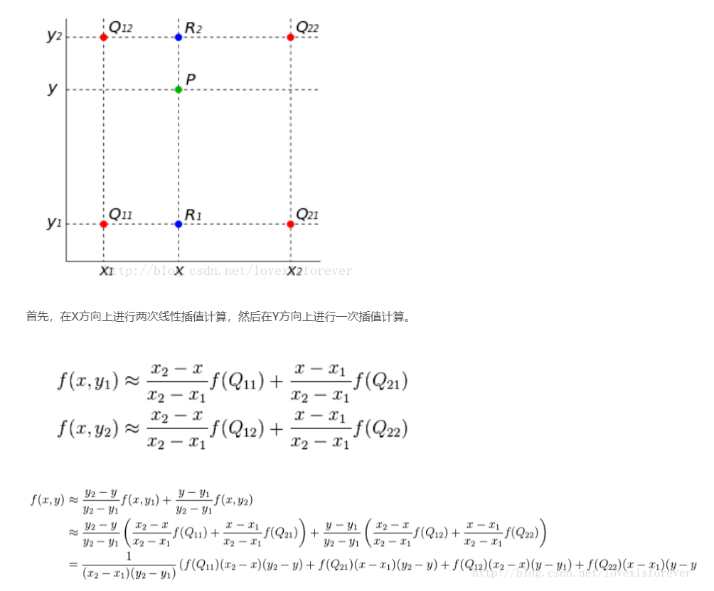
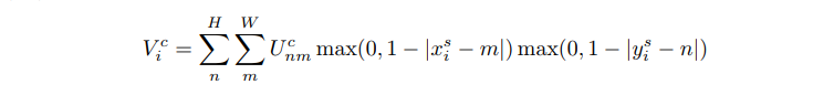
3、Sampler:根据原图片和Grid generator产生的采样网格,使用双线性插值生成输出目标图片。双线性插值其实就是进行了三次简单的线性插值计算,原理如下
整理为更简洁的公式:f(i+u,j+v) = (1-u)(1-v)f(i,j) + (1-u)vf(i,j+1) + u(1-v)f(i+1,j) + uvf(i+1,j+1)
比如对于坐标为[1.6,2.4]的像素值:
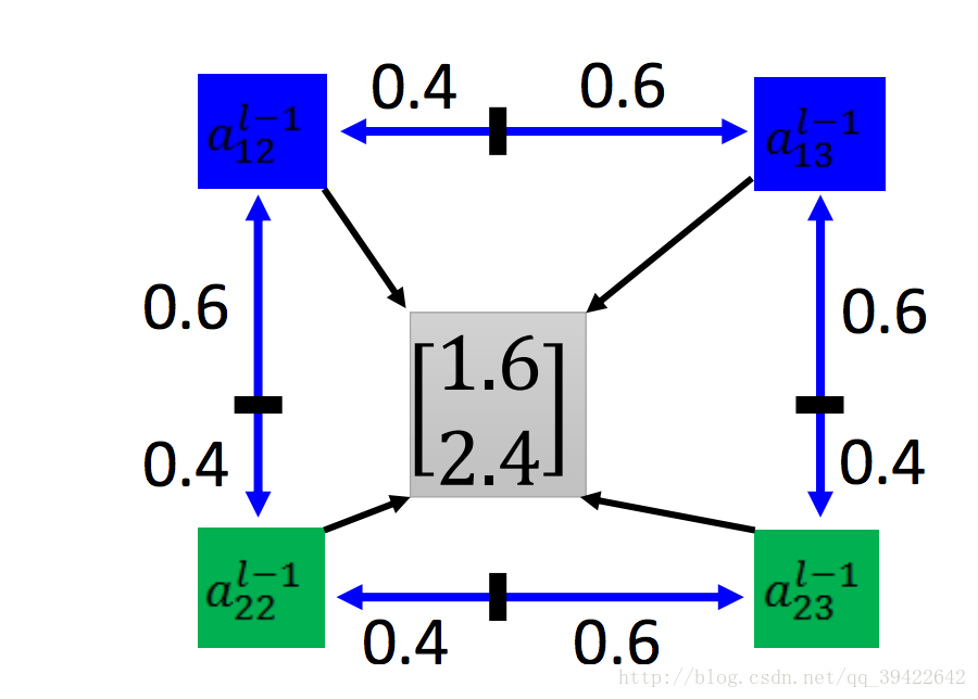
计算公式为:
f(1+0.6,2+0.4) = (1-0.6) x (1-0.4) x f(1,2) + (1-0.6) x 0.4 x f(1,3) + 0.6 x (1-0.4) x f(2,2) + 0.6 x 0.4 x f(2,3)
在论文中,作者给出的计算公式为:
前向过程
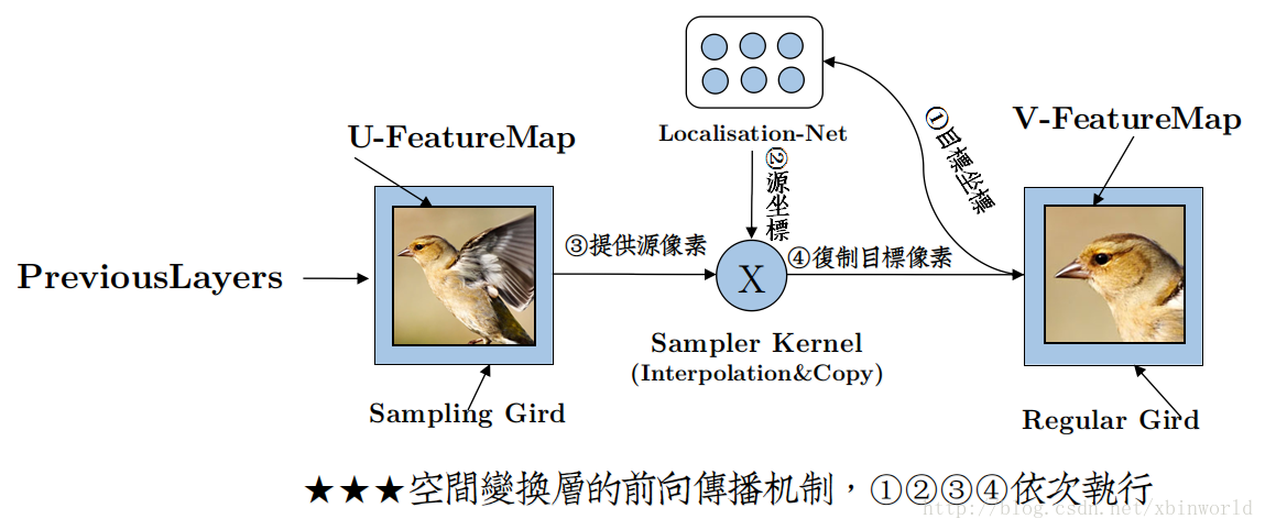
上图展示了一个STN前向传播的完整过程,下面通过部分tensorflow实现代码来理解STN的原理。
Tensorflow部分实现代码
STN整体过程:
import tensorflow as tf

def spatial_transformer_network(input_fmap, theta, out_dims=None, **kwargs):
    """
    The layer is composed of 3 elements:
    - localization_net: takes the original image as input and outputs
      the parameters of the affine transformation that should be applied
      to the input image. 输入原图,输出一个需要学习参数的2x3变换矩阵
    - affine_grid_generator: generates a grid of (x,y) coordinates that
      correspond to a set of points where the input should be sampled
      to produce the transformed output. 生成一个网格(x,y)坐标,对应了一组点,
      即为了生成变换后的输出,应该去原图片的哪些点去采样
    - bilinear_sampler: takes as input the original image and the grid
      and produces the output image using bilinear interpolation.
      根据原图和之前生成的网格,使用双线性插值生成输出图片
    Input
    -----
    - input_fmap: output of the previous layer. Can be input if spatial
      transformer layer is at the beginning of architecture. Should be
      a tensor of shape (B, H, W, C).
    - theta: affine transform tensor of shape (B, 6). Permits cropping,
      translation and isotropic scaling. Initialize to identity matrix.
      It is the output of the localization network.
    Returns
    -------
    - out_fmap: transformed input feature map. Tensor of size (B, H, W, C).
    Notes
    -----
    'Spatial Transformer Networks', Jaderberg et. al,
         (https://arxiv.org/abs/1506.02025)
    """
    # grab input dimensions
    B = tf.shape(input_fmap)[0]
    H = tf.shape(input_fmap)[1]
    W = tf.shape(input_fmap)[2]

    # reshape theta to (B, 2, 3)
    theta = tf.reshape(theta, [B, 2, 3])

    # generate grids of same size or upsample/downsample if specified
    if out_dims:
        out_H = out_dims[0]
        out_W = out_dims[1]
        batch_grids = affine_grid_generator(out_H, out_W, theta)
    else:
        batch_grids = affine_grid_generator(H, W, theta)

    x_s = batch_grids[:, 0, :, :]
    y_s = batch_grids[:, 1, :, :]

    # sample input with grid to get output
    out_fmap = bilinear_sampler(input_fmap, x_s, y_s)

    return out_fmap
生成网格过程:
def affine_grid_generator(height, width, theta):
    """
    This function returns a sampling grid, which when
    used with the bilinear sampler on the input feature
    map, will create an output feature map that is an
    affine transformation [1] of the input feature map.
    Input
    -----
    - height: desired height of grid/output. Used
      to downsample or upsample.
    - width: desired width of grid/output. Used
      to downsample or upsample.
    - theta: affine transform matrices of shape (num_batch, 2, 3).
      For each image in the batch, we have 6 theta parameters of
      the form (2x3) that define the affine transformation T.
    Returns
    -------
    - normalized grid (-1, 1) of shape (num_batch, 2, H, W).
      The 2nd dimension has 2 components: (x, y) which are the
      sampling points of the original image for each point in the
      target image.
    Note
    ----
    [1]: the affine transformation allows cropping, translation,
         and isotropic scaling.
    """
    num_batch = tf.shape(theta)[0]

    # create normalized 2D grid
    x = tf.linspace(-1.0, 1.0, width)
    y = tf.linspace(-1.0, 1.0, height)
    x_t, y_t = tf.meshgrid(x, y)

    # flatten
    x_t_flat = tf.reshape(x_t, [-1])
    y_t_flat = tf.reshape(y_t, [-1])

    # reshape to [x_t, y_t , 1] - (homogeneous form)
    ones = tf.ones_like(x_t_flat)
    sampling_grid = tf.stack([x_t_flat, y_t_flat, ones])

    # repeat grid num_batch times
    sampling_grid = tf.expand_dims(sampling_grid, axis=0)
    sampling_grid = tf.tile(sampling_grid, tf.stack([num_batch, 1, 1]))

    # cast to float32 (required for matmul)
    theta = tf.cast(theta, 'float32')
    sampling_grid = tf.cast(sampling_grid, 'float32')

    # transform the sampling grid - batch multiply
    batch_grids = tf.matmul(theta, sampling_grid)
    # batch grid has shape (num_batch, 2, H*W)

    # reshape to (num_batch, H, W, 2)
    batch_grids = tf.reshape(batch_grids, [num_batch, 2, height, width])

    return batch_grids
根据网格采样的过程:
def bilinear_sampler(img, x, y):
    """
    Performs bilinear sampling of the input images according to the
    normalized coordinates provided by the sampling grid. Note that
    the sampling is done identically for each channel of the input.
    To test if the function works properly, output image should be
    identical to input image when theta is initialized to identity
    transform.
    Input
    -----
    - img: batch of images in (B, H, W, C) layout.
    - grid: x, y which is the output of affine_grid_generator.
    Returns
    -------
    - out: interpolated images according to grids. Same size as grid.
    """
    H = tf.shape(img)[1]
    W = tf.shape(img)[2]
    max_y = tf.cast(H - 1, 'int32')
    max_x = tf.cast(W - 1, 'int32')
    zero = tf.zeros([], dtype='int32')

    # rescale x and y to [0, W-1/H-1]
    x = tf.cast(x, 'float32')
    y = tf.cast(y, 'float32')
    x = 0.5 * ((x + 1.0) * tf.cast(max_x-1, 'float32'))
    y = 0.5 * ((y + 1.0) * tf.cast(max_y-1, 'float32'))

    # grab 4 nearest corner points for each (x_i, y_i)
    x0 = tf.cast(tf.floor(x), 'int32')
    x1 = x0 + 1
    y0 = tf.cast(tf.floor(y), 'int32')
    y1 = y0 + 1

    # clip to range [0, H-1/W-1] to not violate img boundaries
    x0 = tf.clip_by_value(x0, zero, max_x)
    x1 = tf.clip_by_value(x1, zero, max_x)
    y0 = tf.clip_by_value(y0, zero, max_y)
    y1 = tf.clip_by_value(y1, zero, max_y)

    # get pixel value at corner coords
    Ia = get_pixel_value(img, x0, y0)
    Ib = get_pixel_value(img, x0, y1)
    Ic = get_pixel_value(img, x1, y0)
    Id = get_pixel_value(img, x1, y1)

    # recast as float for delta calculation
    x0 = tf.cast(x0, 'float32')
    x1 = tf.cast(x1, 'float32')
    y0 = tf.cast(y0, 'float32')
    y1 = tf.cast(y1, 'float32')

    # calculate deltas
    wa = (x1-x) * (y1-y)
    wb = (x1-x) * (y-y0)
    wc = (x-x0) * (y1-y)
    wd = (x-x0) * (y-y0)

    # add dimension for addition
    wa = tf.expand_dims(wa, axis=3)
    wb = tf.expand_dims(wb, axis=3)
    wc = tf.expand_dims(wc, axis=3)
    wd = tf.expand_dims(wd, axis=3)

    # compute output
    out = tf.add_n([wa*Ia, wb*Ib, wc*Ic, wd*Id])

    return out
实验结果
Distorted MNIST
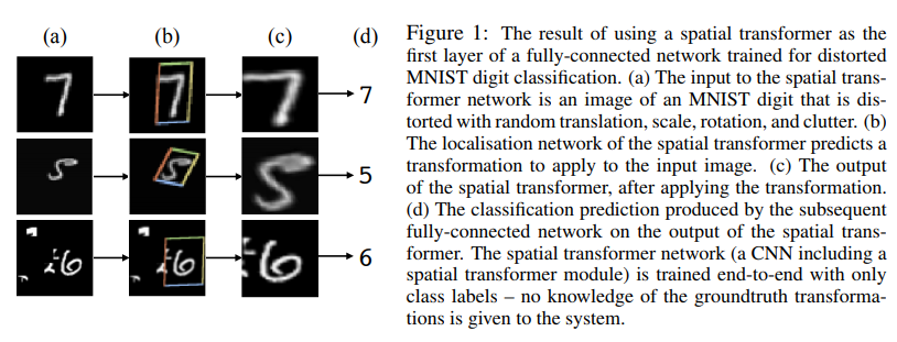
如上图,可以看到STN如何帮助网络精准的学习到健壮的分类模型,通过放缩和消除背景影响,定位关键信息,再做标准化操作。
German Traffic Sign Recognition Benchmark (GTSRB) dataset
可以看到空间变换会集中于关键信息上,移除了背景信息。
总的来说,STN通过把旋转、平移和缩放显式地添加到了网络的学习过程,更有利于End-to-end网络地学习,并且对于上述干扰条件下地输入,网络仍能保持较好的输出结果。
参考博客:https://blog.csdn.net/qq_39422642/article/details/78870629
https://blog.csdn.net/xbinworld/article/details/69049680
https://blog.csdn.net/u011974639/article/details/79681455
发布者:全栈程序员-站长,转载请注明出处:https://javaforall.net/180319.html原文链接:https://javaforall.net


