大家好，又见面了，我是你们的朋友全栈君。如果您正在找激活码,请点击查看最新教程,关注关注公众号 “全栈程序员社区” 获取激活教程,可能之前旧版本教程已经失效.最新Idea2022.1教程亲测有效,一键激活。

Jetbrains全系列IDE稳定放心使用

空间变换网络(Spatial Transformer Network)

本文的参考文献为：《Spatial Transformer Networks》

卷积神经网络定义了一个异常强大的模型类，但在计算和参数有效的方式下仍然受限于对输入数据的空间不变性。在此引入了一个新的可学模块，空间变换网络，它显式地允许在网络中对数据进行空间变换操作。这个可微的模块可以插入到现有的卷积架构中，使神经网络能够主动地在空间上转换特征映射，在特征映射本身上有条件，而不需要对优化过程进行额外的训练监督或修改。我们展示了空间变形的使用结果，在模型中学习了平移、缩放、旋转和更一般的扭曲，结果在几个基准上得到了很好的效果。

空间变换器(Spatial Transformers)

一个空间变换器的运作机制可以分为三个部分，如下图所示：1） 本地网络（Localisation Network）；2）网格生成器( Grid Genator)；3）采样器（Sampler）。

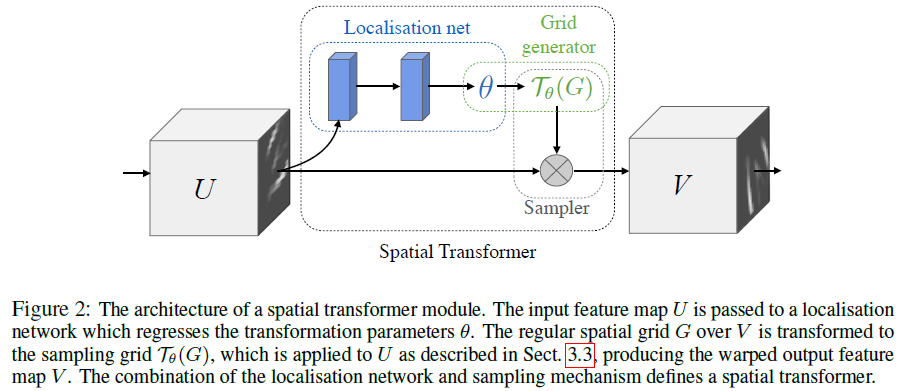
本地网络是一个用来回归变换参数$\theta$的网络，它的输入时特征图像，然后经过一系列的隐藏网络层（全连接或者卷积网，再加一个回归层）输出空间变换参数。$\theta$的形式可以多样，如需实现2D仿射变换，$\theta$ 就是一个6维（2×3）向量的输出。$\theta$的尺寸大小依赖于变换的类型。

$$\theta = f_{loc}(U)$$

网格生成器（Grid Generator）是依据预测的变换参数来构建一个采样网格，它是一组输入图像中的点经过采样变换后得到的输出。网格生成器其实得到的是一种映射关系$\mathcal T_\theta$。假设特征图像$U$每个像素的坐标为$(x^s_i,y^s_i)$， $V$ 的每个像素坐标为$(x^t_i,y^t_i)$, 空间变换函数 $\mathcal T_\theta$ 为二维仿射变换函数，那么 $(x^s_i,y^s_i)$和$(x^t_i,y^t_i)$的对应关系可以写为：

$$\begin{pmatrix}x_i^s \\ y_i^s\end{pmatrix} =\mathcal T_\theta(G_i)=\mathbf{A}_\theta\begin{pmatrix}x_i^t \\ y_i^t\\1\\\end{pmatrix}=\begin{bmatrix}\theta_{11}&\theta_{12}&\theta_{13}\\ \theta_{21}&\theta_{22}&\theta_{23}\\ \end{bmatrix}\begin{pmatrix}x_i^t \\ y_i^t\\1\\\end{pmatrix}$$

采样器利用采样网格和输入的特征图同时作为输入产生输出，得到了特征图经过变换之后的结果。

$$V_i^c=\sum_n^{H}{\sum_m^{W}{ U^c_{nm} \max(0, 1-|x_i^s-m|)\max(0, 1-|y_i^s-n|)}}$$

至此，整个前向传播就完成了。与以往的网络稍微不同的就是STN中有一个采样（插值）的过程，这个采样需要依靠一个特定的网格作为引导。但是细想，我们常用的池化也是一种采样（插值）方式，只不过使用的网格有点特殊而已。

既然存在网络，需要训练，那么就必须得考虑损失的反向传播了。对于自己定义的sampler，这里的反向传播公式需要推导。
其中，输出对采样器的求导公式为：

$$\frac{\partial{V_i^c}}{\partial{U^c_{nm}}}=\sum_n^{H}{\sum_m^{W}{ \max(0, 1-|x_i^s-m|)\max(0, 1-|y_i^s-n|)}} \\\frac{\partial{V_i^c}}{\partial{x^s_i}}=\sum_n^{H}{\sum_m^{W}{ U^c_{nm} \max(0, 1-|x_i^s-m|}}\begin{cases}0, & \text{if $|m-x_i^s|\ge1$} \\1, & \text{if $m\ge{x_i^s}$}\\-1 & \text{if $m\lt{x_i^s}$}\\\end{cases}\\\frac{\partial{V_i^c}}{\partial{y^s_i}}=\sum_n^{H}{\sum_m^{W}{ U^c_{nm} \max(0, 1-|y_i^s-n|)}}\begin{cases}0, & \text{if $|n-y_i^s|\ge1$} \\1, & \text{if $n\ge{y_i^s}$}\\-1 & \text{if $n\lt{y_i^s}$}\\\end{cases}$$

输出对grid generator的求导公式需要依据使用的变换公式自行确定，但大体公式如下计算：

$$\frac{\partial{V_i^c}}{\partial{\theta}}= \begin{pmatrix}\frac{\partial{V_i^c}}{\partial{x^s_i}} \cdot \frac{\partial{x^s_i}}{\partial{\theta}} \\ \frac{\partial{V_i^c}}{\partial{y^s_i}} \cdot \frac{\partial{y^s_i}}{\partial{\theta}} \end{pmatrix}$$

将以上部分组合在一起就能构成STN网络了。

pytorch 源码

# -*- coding: utf-8 -*-
""" Spatial Transformer Networks Tutorial ===================================== **Author**: `Ghassen HAMROUNI <https://github.com/GHamrouni>`_ .. figure:: /_static/img/stn/FSeq.png In this tutorial, you will learn how to augment your network using a visual attention mechanism called spatial transformer networks. You can read more about the spatial transformer networks in the `DeepMind paper <https://arxiv.org/abs/1506.02025>`__ Spatial transformer networks are a generalization of differentiable attention to any spatial transformation. Spatial transformer networks (STN for short) allow a neural network to learn how to perform spatial transformations on the input image in order to enhance the geometric invariance of the model. For example, it can crop a region of interest, scale and correct the orientation of an image. It can be a useful mechanism because CNNs are not invariant to rotation and scale and more general affine transformations. One of the best things about STN is the ability to simply plug it into any existing CNN with very little modification. """
# License: BSD
# Author: Ghassen Hamrouni

from __future__ import print_function
import torch
import torch.nn as nn
import torch.nn.functional as F
import torch.optim as optim
import torchvision
from torchvision import datasets, transforms
import matplotlib.pyplot as plt
import numpy as np

plt.ion()   # interactive mode

######################################################################
# Loading the data
# ----------------
#
# In this post we experiment with the classic MNIST dataset. Using a
# standard convolutional network augmented with a spatial transformer
# network.

device = torch.device("cuda" if torch.cuda.is_available() else "cpu")

# Training dataset
train_loader = torch.utils.data.DataLoader(
    datasets.MNIST(root='.', train=True, download=True,
                   transform=transforms.Compose([
                       transforms.ToTensor(),
                       transforms.Normalize((0.1307,), (0.3081,))
                   ])), batch_size=64, shuffle=True, num_workers=4)
# Test dataset
test_loader = torch.utils.data.DataLoader(
    datasets.MNIST(root='.', train=False, transform=transforms.Compose([
        transforms.ToTensor(),
        transforms.Normalize((0.1307,), (0.3081,))
    ])), batch_size=64, shuffle=True, num_workers=4)

######################################################################
# Depicting spatial transformer networks
# --------------------------------------
#
# Spatial transformer networks boils down to three main components :
#
# - The localization network is a regular CNN which regresses the
# transformation parameters. The transformation is never learned
# explicitly from this dataset, instead the network learns automatically
# the spatial transformations that enhances the global accuracy.
# - The grid generator generates a grid of coordinates in the input
# image corresponding to each pixel from the output image.
# - The sampler uses the parameters of the transformation and applies
# it to the input image.
#
# .. figure:: /_static/img/stn/stn-arch.png
#
# .. Note::
# We need the latest version of PyTorch that contains
# affine_grid and grid_sample modules.
#


class Net(nn.Module):
    def __init__(self):
        super(Net, self).__init__()
        self.conv1 = nn.Conv2d(1, 10, kernel_size=5)
        self.conv2 = nn.Conv2d(10, 20, kernel_size=5)
        self.conv2_drop = nn.Dropout2d()
        self.fc1 = nn.Linear(320, 50)
        self.fc2 = nn.Linear(50, 10)

        # Spatial transformer localization-network
        self.localization = nn.Sequential(
            nn.Conv2d(1, 8, kernel_size=7),
            nn.MaxPool2d(2, stride=2),
            nn.ReLU(True),
            nn.Conv2d(8, 10, kernel_size=5),
            nn.MaxPool2d(2, stride=2),
            nn.ReLU(True)
        )

        # Regressor for the 3 * 2 affine matrix
        self.fc_loc = nn.Sequential(
            nn.Linear(10 * 3 * 3, 32),
            nn.ReLU(True),
            nn.Linear(32, 3 * 2)
        )

        # Initialize the weights/bias with identity transformation
        self.fc_loc[2].weight.data.zero_()
        self.fc_loc[2].bias.data.copy_(torch.tensor([1, 0, 0, 0, 1, 0], dtype=torch.float))

    # Spatial transformer network forward function
    def stn(self, x):
        xs = self.localization(x)
        xs = xs.view(-1, 10 * 3 * 3)
        theta = self.fc_loc(xs)
        theta = theta.view(-1, 2, 3)

        grid = F.affine_grid(theta, x.size())
        x = F.grid_sample(x, grid)

        return x

    def forward(self, x):
        # transform the input
        x = self.stn(x)

        # Perform the usual forward pass
        x = F.relu(F.max_pool2d(self.conv1(x), 2))
        x = F.relu(F.max_pool2d(self.conv2_drop(self.conv2(x)), 2))
        x = x.view(-1, 320)
        x = F.relu(self.fc1(x))
        x = F.dropout(x, training=self.training)
        x = self.fc2(x)
        return F.log_softmax(x, dim=1)


model = Net().to(device)

######################################################################
# Training the model
# ------------------
#
# Now, let's use the SGD algorithm to train the model. The network is
# learning the classification task in a supervised way. In the same time
# the model is learning STN automatically in an end-to-end fashion.


optimizer = optim.SGD(model.parameters(), lr=0.01)


def train(epoch):
    model.train()
    for batch_idx, (data, target) in enumerate(train_loader):
        data, target = data.to(device), target.to(device)

        optimizer.zero_grad()
        output = model(data)
        loss = F.nll_loss(output, target)
        loss.backward()
        optimizer.step()
        if batch_idx % 500 == 0:
            print('Train Epoch: {} [{}/{} ({:.0f}%)]\tLoss: {:.6f}'.format(
                epoch, batch_idx * len(data), len(train_loader.dataset),
                100. * batch_idx / len(train_loader), loss.item()))
#
# A simple test procedure to measure STN the performances on MNIST.
#


def test():
    with torch.no_grad():
        model.eval()
        test_loss = 0
        correct = 0
        for data, target in test_loader:
            data, target = data.to(device), target.to(device)
            output = model(data)

            # sum up batch loss
            test_loss += F.nll_loss(output, target, size_average=False).item()
            # get the index of the max log-probability
            pred = output.max(1, keepdim=True)[1]
            correct += pred.eq(target.view_as(pred)).sum().item()

        test_loss /= len(test_loader.dataset)
        print('\nTest set: Average loss: {:.4f}, Accuracy: {}/{} ({:.0f}%)\n'
              .format(test_loss, correct, len(test_loader.dataset),
                      100. * correct / len(test_loader.dataset)))

######################################################################
# Visualizing the STN results
# ---------------------------
#
# Now, we will inspect the results of our learned visual attention
# mechanism.
#
# We define a small helper function in order to visualize the
# transformations while training.


def convert_image_np(inp):
    """Convert a Tensor to numpy image."""
    inp = inp.numpy().transpose((1, 2, 0))
    mean = np.array([0.485, 0.456, 0.406])
    std = np.array([0.229, 0.224, 0.225])
    inp = std * inp + mean
    inp = np.clip(inp, 0, 1)
    return inp

# We want to visualize the output of the spatial transformers layer
# after the training, we visualize a batch of input images and
# the corresponding transformed batch using STN.


def visualize_stn():
    with torch.no_grad():
        # Get a batch of training data
        data = next(iter(test_loader))[0].to(device)

        input_tensor = data.cpu()
        transformed_input_tensor = model.stn(data).cpu()

        in_grid = convert_image_np(
            torchvision.utils.make_grid(input_tensor))

        out_grid = convert_image_np(
            torchvision.utils.make_grid(transformed_input_tensor))

        # Plot the results side-by-side
        f, axarr = plt.subplots(1, 2)
        axarr[0].imshow(in_grid)
        axarr[0].set_title('Dataset Images')

        axarr[1].imshow(out_grid)
        axarr[1].set_title('Transformed Images')


for epoch in range(1, 20 + 1):
    train(epoch)
    test()

# Visualize the STN transformation on some input batch
visualize_stn()

plt.ioff()
plt.show()

Reference

[1] 【论文笔记】Spatial Transformer Networks
[2] Spatial Transformer Networks Tutorial